pith. sign in

arxiv: 2605.21684 · v1 · pith:B5IKPYMWnew · submitted 2026-05-20 · 🌌 astro-ph.EP · astro-ph.HE

Bayesian Modeling of NICER Cometary X-ray Spectra: A Legacy Survey of Solar-Wind Charge Exchange

Pith reviewed 2026-05-22 08:10 UTC · model grok-4.3

classification 🌌 astro-ph.EP astro-ph.HE
keywords cometsX-ray spectroscopysolar wind charge exchangeNICERBayesian modelingfreeze-in temperaturessolar wind variability
0
0 comments X

The pith

Bayesian modeling of NICER comet spectra separates carbon-derived solar-wind freeze-in temperatures at 1.4-1.7 MK from higher nitrogen- and oxygen-derived values at 2.0-2.3 MK.

A machine-rendered reading of the paper's core claim, the machinery that carries it, and where it could break.

The paper performs a uniform analysis of soft X-ray data from eight comets observed by NICER. It applies Bayesian statistics to identify charge-exchange emission lines, measure relative ion fluxes, and derive solar-wind freeze-in temperatures from different elements. The results show recurring spectral families and a clear separation in inferred temperatures by element. Short-term variability in these temperatures is linked to changes in the solar wind rather than comet properties. The work also discusses modeling limitations and calls for better laboratory data and high-resolution observations.

Core claim

Epoch-resolved flux ratios from the NICER spectra produce a robust separation between diagnostics, with carbon-derived freeze-in temperatures clustering near 1.4-1.7 MK while nitrogen- and oxygen-derived diagnostics are systematically higher at typically 2.0-2.3 MK; short-timescale variability in the inferred conditions is common and attributed to instantaneous solar-wind charge-state fluctuations rather than large changes in coma composition.

What carries the argument

Bayesian fitting of charge-exchange line components using physically motivated priors and model selection to extract relative ion fluxes and infer nominal solar-wind freeze-in temperatures from low-resolution spectra.

If this is right

  • Spectral morphologies of cometary X-rays fall into distinct carbon-dominated, intermediate, and nitrogen-oxygen-dominated families.
  • Instantaneous solar-wind charge-state fluctuations dominate observed spectral differences over changes in coma composition.
  • Bayesian model selection with priors mitigates degeneracies that affect low-resolution inferences of ion populations.
  • Laboratory measurements of charge-exchange cross sections are needed to refine the temperature diagnostics.
  • Coordinated high-resolution X-ray observations would help validate the low-resolution results.

Where Pith is reading between the lines

These are editorial extensions of the paper, not claims the author makes directly.

  • Multi-element line ratios provide a practical way to monitor solar-wind conditions even with modest spectral resolution.
  • The observed separation suggests that single-element diagnostics may systematically misrepresent the average solar-wind state sampled by comets.
  • The same Bayesian approach could be extended to X-ray observations of other solar-system objects that interact with the solar wind.

Load-bearing premise

The mapping from observed line flux ratios to freeze-in temperatures assumes that the charge-exchange cross sections and the underlying solar-wind ion populations are correctly described by the chosen atomic database and model priors without significant contamination from other emission processes.

What would settle it

A new set of observations or laboratory measurements that shows the carbon and nitrogen-oxygen line ratios do not produce separated temperature clusters or that reveals substantial contamination from non-charge-exchange processes would falsify the reported separation and variability attribution.

Figures

Figures reproduced from arXiv: 2605.21684 by Damian J. Christian, Dennis Bodewits, Dusan Odstrcil, Konrad Dennerl, Steven Bromley, T. K. Deskins.

Figure 1
Figure 1. Figure 1: Heliocentric latitude projection of observed comet positions on their respective observation dates. The Sun is at the origin and the dashed grey line marks the ecliptic plane. Each comet is plotted at 𝑥 = 𝑟 cos 𝛽, 𝑦 = 𝑟 sin 𝛽 (with 𝑟 the heliocentric distance in AU and 𝛽 the heliocentric ecliptic latitude). Letters mark observations and correspond to:(A1) C/2017 T2: 2020-04-24; (A2) C/2017 T2: 2020-06-26; … view at source ↗
Figure 2
Figure 2. Figure 2: X-ray spectrum from the interaction between the solar wind and the atmospheres of 12P/Pons-Brooks (left) and C/2017 K2 (PANSTARRS) (right), each dataset fitted with the Bayesian Color Model (BCM). The BCM utilizes Bayesian prin￾ciples to quantitatively determine optimal parameters for fitting the low-resolution data. By iterating through peak combinations associated with C v, C vi, N vi, N vii, O vii, O vi… view at source ↗
Figure 3
Figure 3. Figure 3: Top: X-ray spectrum for the full 62P/Tsuchinshan dataset from the solar wind’s interaction with the atmosphere of comet 62P/Tsuchinshan, fitted with the Bayesian Color Model (BCM), which uses the Bayesian Information Criterion (BIC) as a model-selection tool to balance model complexity and goodness of fit. We only consider energies between 370 eV and 900 eV because no lines are fitted above 900 eV. Colored… view at source ↗
Figure 4
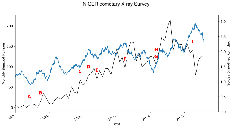
Figure 4. Figure 4: Monthly sunspot number (black) between 2020-01-01 and 2025-12-31 with observation annotations (red letters) marking representative NICER on-comet observation dates: (A) C/2017 T2 (PANSTARRS): 2020-05-24; (B) 88P/Howell: 2020- 10-01; (C) 67P/Churyumov–Gerasimenko: 2021-11-30; (D) 19P/Borrelly: 2022-02-15; (E) C/2017 K2 (PANSTARRS): 2022-06- 15; (F) C/2022 E3 (ZTF): 2023-03-21; (G) 62P/Tsuchinshan: 2024-02-2… view at source ↗
Figure 5
Figure 5. Figure 5: Simulated solar-wind parameters from the ENLIL model with GONG boundary conditions, evaluated at the position of Comet 19P/Borrelly in January (left) and February (right) 2022. The horizontal panels display the velocity (𝑉𝑟 ), density (𝑁), temperature (𝑇 ), and magnetic field intensity (|𝐵|) of the solar wind. K Shocks are marked by vertical blue lines with annotated times, while coronal mass ejections are… view at source ↗
Figure 6
Figure 6. Figure 6: An X-ray spectrum shown between 0.37-2.00 keV is shown from one representative observation. The y-axis shows the normalized count rate, and the x-axis shows energy. The on-target observation is depicted in black, while the weighted average of pre- and post-background observations is presented in solid red. The dotted red line is the Xspec-fitted model of our empirical background measurements, while the pin… view at source ↗
Figure 7
Figure 7. Figure 7: X-ray spectrum for the full dataset for C/2022 E3 (ZTF). The black data series is the spectrum before background subtraction; the purple data series is the average of the pre-comet and post-comet background spectra, which dominates above 1 keV; the green data series is the spectrum attributable to the comet after background subtraction. The average background flux for the pre-comet and post-comet backgroun… view at source ↗
Figure 8
Figure 8. Figure 8: Freeze-in temperatures for comet C/2017 K2 (PANSTARRS) inferred from flux ratios, plotted versus observing epoch. Blue shows 𝑇f reeze derived from C vi / C v, green is from N vii / N vi, and red is from O viii / O vii; vertical bars are 1𝜎 uncertainties propagated from the line-fit errors. 88P exhibits significant epoch-to-epoch variability in its freeze-in diagnostics. The full-dataset diagnostics are 𝑇f … view at source ↗
Figure 9
Figure 9. Figure 9: Freeze-in temperature inferred from the O viii / O vii flux ratio plotted against the measured oxygen flux ratio for each comet and observing epoch. Vertical error bars show 1-𝜎 uncertainties propagated from the line-fit errors. Colors identify comets: T2 (brown), 88P (magenta), 67P (purple), 19P (orange), K2 (blue), E3 (red), and 62P (green). Marker shapes denote observing epochs: circle = Epoch 1, X = Ep… view at source ↗
Figure 10
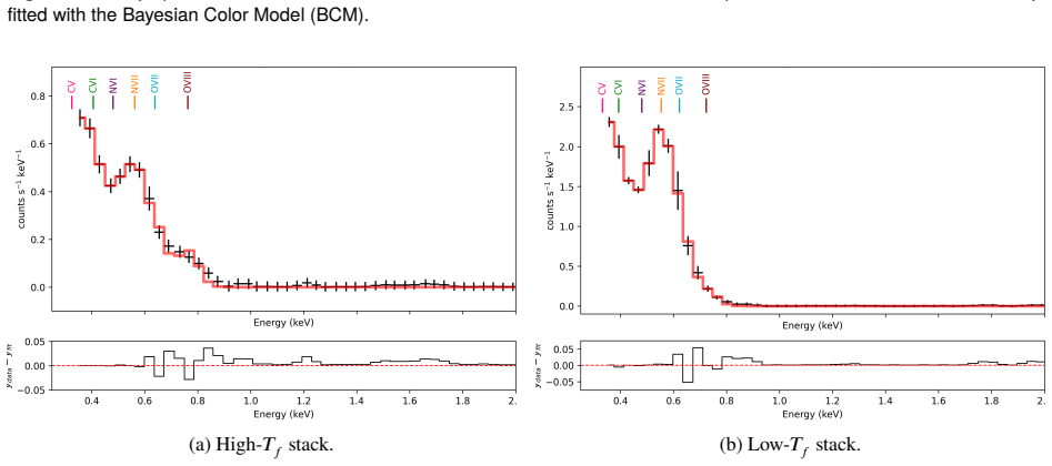
Figure 10. Figure 10: X-ray spectrum from the interaction between the solar wind and the atmospheres of all nine comets in the study, fitted with the Bayesian Color Model (BCM). (a) High-𝑇𝑓 stack. (b) Low-𝑇𝑓 stack [PITH_FULL_IMAGE:figures/full_fig_p022_10.png] view at source ↗
Figure 11
Figure 11. Figure 11: X-ray spectra from the interaction between the solar wind and the atmospheres of comets, separated by freeze-in temperature (𝑇𝑓 ). Left: spectrum for the high 𝑇𝑓 stack. Right: spectrum for the low 𝑇𝑓 stack. Both spectra are fitted with the Bayesian Color Model (BCM). The classification of epochs into high-𝑇𝑓 and low-𝑇𝑓 groups is based specifically on the oxygen flux ratio, 𝑂𝐹 𝑅 = O viii / O vii. This choi… view at source ↗
Figure 12
Figure 12. Figure 12: Simulated NICER XTI spectra for cometary charge-exchange interactions, representing a H2O-dominated coma (left) and a CO2 -dominated coma (right). The simulations were performed using the fakeit command in XSPEC with NICER response files from its calibration database. Distinct spectral features arise from different neutral targets, highlighting the compositional dependence of cometary X-ray emission. oxyg… view at source ↗
Figure 13
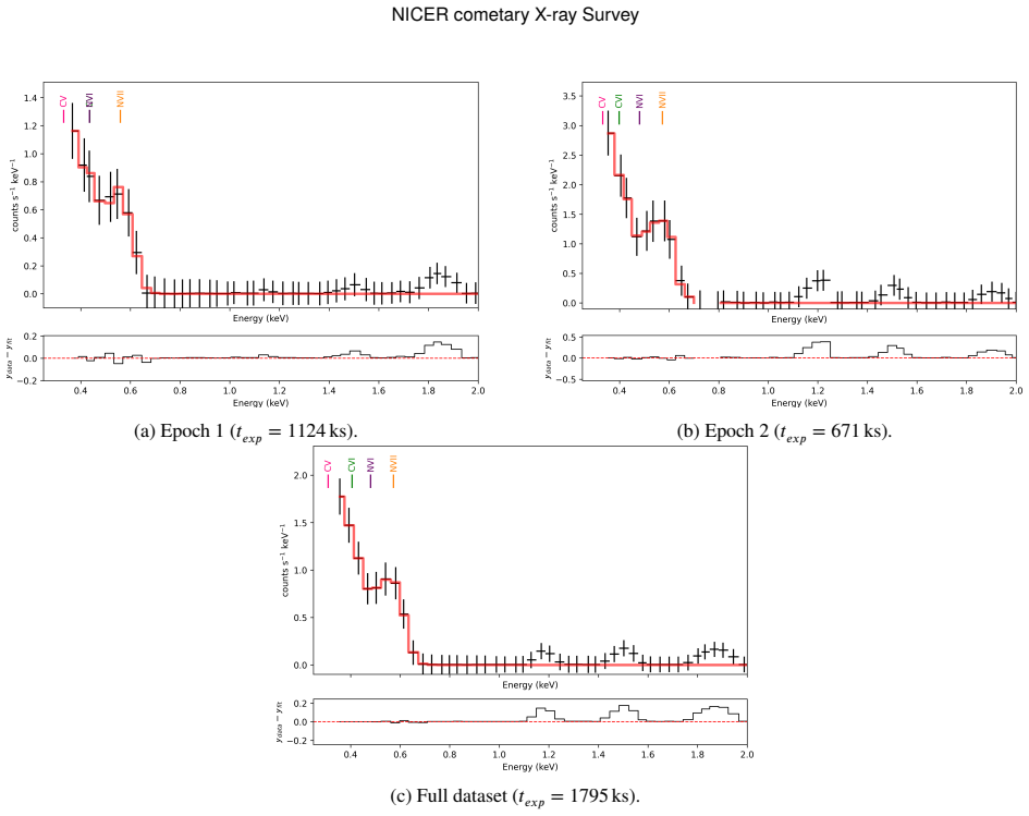
Figure 13. Figure 13: X-ray spectra from the interaction between the solar wind and the atmosphere of C/2017 T2 fitted with the Bayesian Color Model (BCM). B. Spectra This appendix section presents the Bayesian Color Model (BCM) spectral fits for each comet in the survey, showing both spectra from individual observing-epochs and the corresponding full-dataset spectrum and model. The BCM utilizes Bayesian principles to quantita… view at source ↗
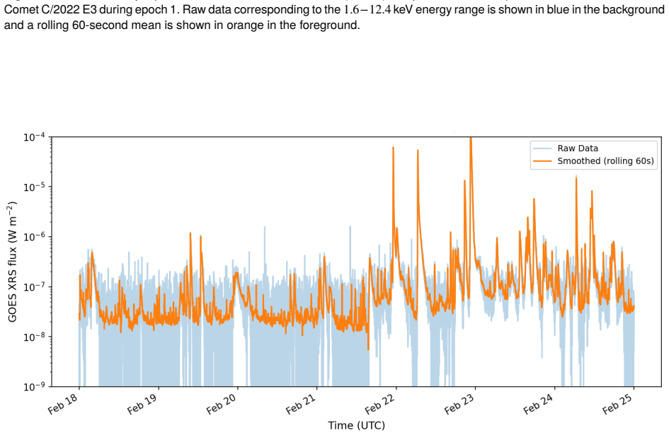
Figure 14
Figure 14. Figure 14: X-ray spectra from the interaction between the solar wind and the atmosphere of 88P/Howell fitted with the Bayesian Color Model (BCM). rolling mean in orange. Each figure covers a single epoch for each comet. These figures illustrate both the day-to-day variability and shorter-term fluctuations in solar X-ray emission over the duration of the observing campaign. T. K. Deskins et al.: Preprint submitted to… view at source ↗
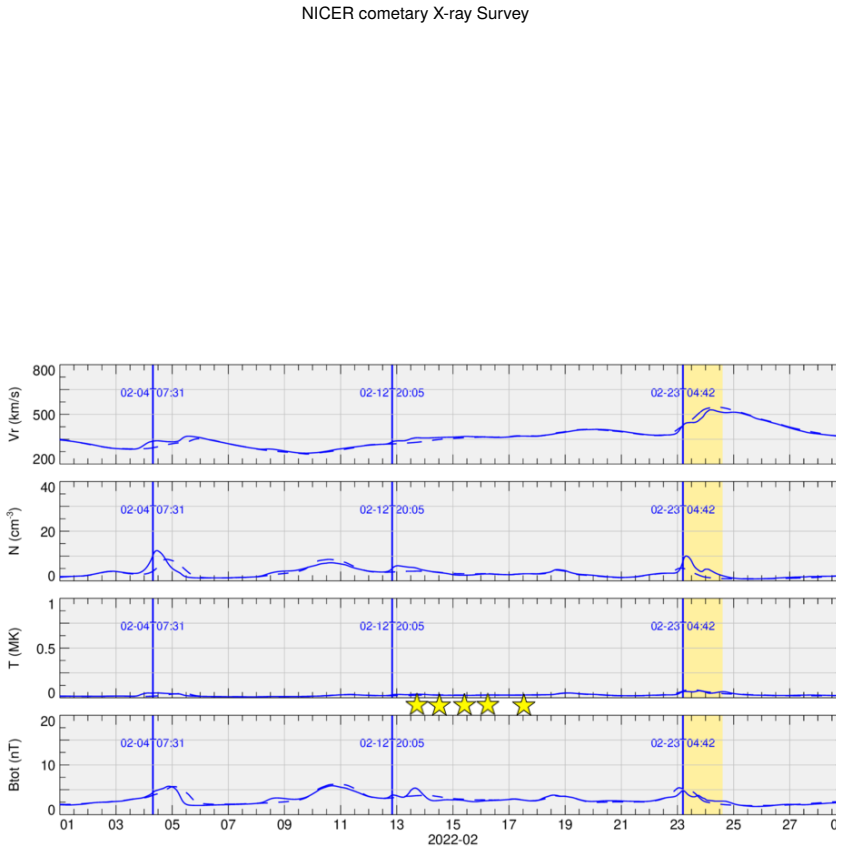
Figure 15
Figure 15. Figure 15: X-ray spectra from the interaction between the solar wind and the atmosphere of 67P/Churyumov–Gerasimenko fitted with the Bayesian Color Model (BCM). T. K. Deskins et al.: Preprint submitted to Elsevier Page 45 of 84 [PITH_FULL_IMAGE:figures/full_fig_p046_15.png] view at source ↗
Figure 16
Figure 16. Figure 16: X-ray spectra from the interaction between the solar wind and the atmosphere of 67P/Churyumov–Gerasimenko fitted with the Bayesian Color Model (BCM). (a) Epoch 1 (𝑡 𝑒𝑥𝑝 = 3583 ks). (b) Epoch 2 (𝑡 𝑒𝑥𝑝 = 6235 ks). (c) Epoch 3 (𝑡 𝑒𝑥𝑝 = 3608 ks). (d) Full dataset (𝑡 𝑒𝑥𝑝 = 13426 ks) [PITH_FULL_IMAGE:figures/full_fig_p047_16.png] view at source ↗
Figure 17
Figure 17. Figure 17: X-ray spectra from the interaction between the solar wind and the atmosphere of 19P/Borrelly fitted with the Bayesian Color Model (BCM). T. K. Deskins et al.: Preprint submitted to Elsevier Page 46 of 84 [PITH_FULL_IMAGE:figures/full_fig_p047_17.png] view at source ↗
Figure 18
Figure 18. Figure 18: X-ray spectra from the interaction between the solar wind and the atmosphere of C/2017 K2 (PANSTARRS) fitted with the Bayesian Color Model (BCM). (a) Epoch 1 (𝑡 𝑒𝑥𝑝 = 16304 ks). (b) Full dataset (𝑡 𝑒𝑥𝑝 = 16304 ks) [PITH_FULL_IMAGE:figures/full_fig_p048_18.png] view at source ↗
Figure 19
Figure 19. Figure 19: X-ray spectra from the interaction between the solar wind and the atmosphere of C/2022 E3 (ZTF) fitted with the Bayesian Color Model (BCM). T. K. Deskins et al.: Preprint submitted to Elsevier Page 47 of 84 [PITH_FULL_IMAGE:figures/full_fig_p048_19.png] view at source ↗
Figure 20
Figure 20. Figure 20: X-ray spectra from the interaction between the solar wind and the atmosphere of 62P/Tsuchinshan fitted with the Bayesian Color Model (BCM). T. K. Deskins et al.: Preprint submitted to Elsevier Page 48 of 84 [PITH_FULL_IMAGE:figures/full_fig_p049_20.png] view at source ↗
Figure 21
Figure 21. Figure 21: X-ray spectra from the interaction between the solar wind and the atmosphere of 12P/Pons–Brooks fitted with the Bayesian Color Model (BCM). (a) Epoch 1 (𝑡 𝑒𝑥𝑝 = 2192 ks). (b) Full dataset (𝑡 𝑒𝑥𝑝 = 2192 ks) [PITH_FULL_IMAGE:figures/full_fig_p050_21.png] view at source ↗
Figure 22
Figure 22. Figure 22: X-ray spectra from the interaction between the solar wind and the atmosphere of P/2010 H2 (Vales) fitted with the Bayesian Color Model (BCM). Given the low quality of the spectra, H2 is not considered in the results. T. K. Deskins et al.: Preprint submitted to Elsevier Page 49 of 84 [PITH_FULL_IMAGE:figures/full_fig_p050_22.png] view at source ↗
Figure 23
Figure 23. Figure 23: Freeze-in temperatures for comet C/2017 T2 inferred from flux ratios, plotted versus observing epoch. Blue shows 𝑇f reeze derived from C vi / C v, green is from N vii / N vi, and red is from O viii / O vii; vertical bars are 1𝜎 uncertainties propagated from the line-fit errors [PITH_FULL_IMAGE:figures/full_fig_p051_23.png] view at source ↗
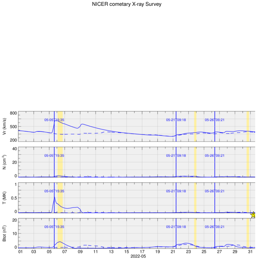
Figure 24
Figure 24. Figure 24: Freeze-in temperatures for comet 88P/Howell inferred from flux ratios, plotted versus observing epoch. Blue shows 𝑇f reeze derived from C vi / C v, green is from N vii / N vi, and red is from O viii / O vii; vertical bars are 1𝜎 uncertainties propagated from the line-fit errors. T. K. Deskins et al.: Preprint submitted to Elsevier Page 50 of 84 [PITH_FULL_IMAGE:figures/full_fig_p051_24.png] view at source ↗
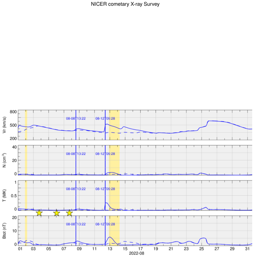
Figure 25
Figure 25. Figure 25: Freeze-in temperatures for comet 67P/Churyumov–Gerasimenko inferred from flux ratios, plotted versus observing epoch. Blue shows 𝑇f reeze derived from C vi / C v, green is from N vii / N vi, and red is from O viii / O vii; vertical bars are 1𝜎 uncertainties propagated from the line-fit errors [PITH_FULL_IMAGE:figures/full_fig_p052_25.png] view at source ↗
Figure 26
Figure 26. Figure 26: Freeze-in temperatures for comet 19P/Borrelly inferred from flux ratios, plotted versus observing epoch. Blue shows 𝑇f reeze derived from C vi / C v, green is from N vii / N vi, and red is from O viii / O vii; vertical bars are 1𝜎 uncertainties propagated from the line-fit errors. T. K. Deskins et al.: Preprint submitted to Elsevier Page 51 of 84 [PITH_FULL_IMAGE:figures/full_fig_p052_26.png] view at source ↗
Figure 27
Figure 27. Figure 27: Freeze-in temperatures for comet C/2017 K2 (PANSTARRS) inferred from flux ratios, plotted versus observing epoch. Blue shows 𝑇f reeze derived from C vi / C v, green is from N vii / N vi, and red is from O viii / O vii; vertical bars are 1𝜎 uncertainties propagated from the line-fit errors [PITH_FULL_IMAGE:figures/full_fig_p053_27.png] view at source ↗
Figure 28
Figure 28. Figure 28: Freeze-in temperatures for comet C/2022 E3 (ZTF) inferred from flux ratios, plotted versus observing epoch. Blue shows 𝑇f reeze derived from C vi / C v, green is from N vii / N vi, and red is from O viii / O vii; vertical bars are 1𝜎 uncertainties propagated from the line-fit errors. T. K. Deskins et al.: Preprint submitted to Elsevier Page 52 of 84 [PITH_FULL_IMAGE:figures/full_fig_p053_28.png] view at source ↗
Figure 29
Figure 29. Figure 29: Freeze-in temperatures for comet 62P/Tsuchinshan inferred from flux ratios, plotted versus observing epoch. Blue shows 𝑇f reeze derived from C vi / C v, green is from N vii / N vi, and red is from O viii / O vii; vertical bars are 1𝜎 uncertainties propagated from the line-fit errors [PITH_FULL_IMAGE:figures/full_fig_p054_29.png] view at source ↗
Figure 30
Figure 30. Figure 30: Freeze-in temperatures for comet 12P/Pons-Brooks inferred from flux ratios, plotted versus observing epoch. Blue shows 𝑇f reeze derived from C vi / C v and green is from N vii / N vi. There is no freeze-in temperature derived from oxygen, as the oxygen pair was not selected by the BCM model for 12P. Vertical bars are 1𝜎 uncertainties propagated from the line-fit errors. T. K. Deskins et al.: Preprint subm… view at source ↗
Figure 31
Figure 31. Figure 31: Simulated solar-wind parameters from the ENLIL model with GONG boundary conditions, evaluated at the position of Comet 67P Churyumov-Gerasimenko in November 2021. The horizontal panels display the velocity (𝑉𝑟 ), density (𝑁), temperature (𝑇 ), and magnetic field intensity (|𝐵|) of the solar wind. K Shocks are marked by vertical blue lines with annotated times, while coronal mass ejections are highlighted … view at source ↗
Figure 32
Figure 32. Figure 32: Simulated solar-wind parameters from the ENLIL model with GONG boundary conditions, evaluated at the position of Comet 67P Churyumov-Gerasimenko in December 2021. The horizontal panels display the velocity (𝑉𝑟 ), density (𝑁), temperature (𝑇 ), and magnetic field intensity (|𝐵|) of the solar wind. K Shocks are marked by vertical blue lines with annotated times, while coronal mass ejections are highlighted … view at source ↗
Figure 33
Figure 33. Figure 33: Simulated solar-wind parameters from the ENLIL model with GONG boundary conditions, evaluated at the position of Comet 19P/Borrelly in January 2022. The horizontal panels display the velocity (𝑉𝑟 ), density (𝑁), temperature (𝑇 ), and magnetic field intensity (|𝐵|) of the solar wind. K Shocks are marked by vertical blue lines with annotated times, while coronal mass ejections are highlighted in yellow. Tim… view at source ↗
Figure 34
Figure 34. Figure 34: Simulated solar-wind parameters from the ENLIL model with GONG boundary conditions, evaluated at the position of Comet 19P/Borrelly in February 2022. The horizontal panels display the velocity (𝑉𝑟 ), density (𝑁), temperature (𝑇 ), and magnetic field intensity (|𝐵|) of the solar wind. K Shocks are marked by vertical blue lines with annotated times, while coronal mass ejections are highlighted in yellow. Ti… view at source ↗
Figure 35
Figure 35. Figure 35: Simulated solar-wind parameters from the ENLIL model with GONG boundary conditions, evaluated at the position of Comet 19P/Borrelly in March 2022. The horizontal panels display the velocity (𝑉𝑟 ), density (𝑁), temperature (𝑇 ), and magnetic field intensity (|𝐵|) of the solar wind. K Shocks are marked by vertical blue lines with annotated times, while coronal mass ejections are highlighted in yellow. Times… view at source ↗
Figure 36
Figure 36. Figure 36: Simulated solar-wind parameters from the ENLIL model with GONG boundary conditions, evaluated at the position of Comet C/2017 K2 (PANSTARRS) in May 2022. The horizontal panels display the velocity (𝑉𝑟 ), density (𝑁), temperature (𝑇 ), and magnetic field intensity (|𝐵|) of the solar wind. K Shocks are marked by vertical blue lines with annotated times, while coronal mass ejections are highlighted in yellow… view at source ↗
Figure 37
Figure 37. Figure 37: Simulated solar-wind parameters from the ENLIL model with GONG boundary conditions, evaluated at the position of Comet C/2017 K2 (PANSTARRS) in June 2022. The horizontal panels display the velocity (𝑉𝑟 ), density (𝑁), temperature (𝑇 ), and magnetic field intensity (|𝐵|) of the solar wind. K Shocks are marked by vertical blue lines with annotated times, while coronal mass ejections are highlighted in yello… view at source ↗
Figure 38
Figure 38. Figure 38: Simulated solar-wind parameters from the ENLIL model with GONG boundary conditions, evaluated at the position of Comet C/2017 K2 (PANSTARRS) in July 2022. The horizontal panels display the velocity (𝑉𝑟 ), density (𝑁), temperature (𝑇 ), and magnetic field intensity (|𝐵|) of the solar wind. K Shocks are marked by vertical blue lines with annotated times, while coronal mass ejections are highlighted in yello… view at source ↗
Figure 39
Figure 39. Figure 39: Simulated solar-wind parameters from the ENLIL model with GONG boundary conditions, evaluated at the position of Comet C/2017 K2 (PANSTARRS) in August 2022. The horizontal panels display the velocity (𝑉𝑟 ), density (𝑁), temperature (𝑇 ), and magnetic field intensity (|𝐵|) of the solar wind. K Shocks are marked by vertical blue lines with annotated times, while coronal mass ejections are highlighted in yel… view at source ↗
Figure 40
Figure 40. Figure 40: Simulated solar-wind parameters from the ENLIL model with GONG boundary conditions, evaluated at the position of Comet C/2022 E3 (ZTF) in March 2023. The horizontal panels display the velocity (𝑉𝑟 ), density (𝑁), temperature (𝑇 ), and magnetic field intensity (|𝐵|) of the solar wind. K Shocks are marked by vertical blue lines with annotated times, while coronal mass ejections are highlighted in yellow. Ti… view at source ↗
Figure 41
Figure 41. Figure 41: Simulated solar-wind parameters from the ENLIL model with GONG boundary conditions, evaluated at the position of Comet 62P/Tsuchinshan in February 2024. The horizontal panels display the velocity (𝑉𝑟 ), density (𝑁), temperature (𝑇 ), and magnetic field intensity (|𝐵|) of the solar wind. K Shocks are marked by vertical blue lines with annotated times, while coronal mass ejections are highlighted in yellow.… view at source ↗
Figure 42
Figure 42. Figure 42: Simulated solar-wind parameters from the ENLIL model with GONG boundary conditions, evaluated at the position of Comet 12P/Pons-Brooks in March 2024. The horizontal panels display the velocity (𝑉𝑟 ), density (𝑁), temperature (𝑇 ), and magnetic field intensity (|𝐵|) of the solar wind. K Shocks are marked by vertical blue lines with annotated times, while coronal mass ejections are highlighted in yellow. Ti… view at source ↗
Figure 43
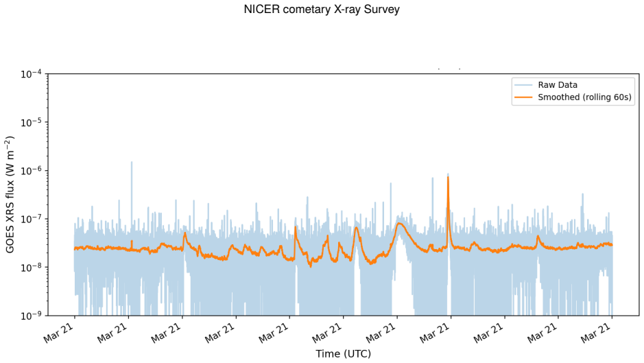
Figure 43. Figure 43: Geostationary Operational Environmental Satellites (GOES) X-ray fluxes over the period of our observations for Comet C/2017 T2. Raw data corresponding to the 1.6 − 12.4 keV energy range is shown in blue in the background and a rolling 60-second mean is shown in orange in the foreground. Our observations were made during each of the periods indicated in the figure. T. K. Deskins et al.: Preprint submitted … view at source ↗
Figure 44
Figure 44. Figure 44: Geostationary Operational Environmental Satellites (GOES) X-ray fluxes over the period of our observations for Comet 88P during epoch 1. Raw data corresponding to the 1.6 − 12.4 keV energy range is shown in blue in the background and a rolling 60-second mean is shown in orange in the foreground. F. Neutral–Species Model Spectra This appendix presents model spectra illustrating the expected differences bet… view at source ↗
Figure 45
Figure 45. Figure 45: Geostationary Operational Environmental Satellites (GOES) X-ray fluxes over the period of our observations for Comet 88P during epoch 2. Raw data corresponding to the 1.6 − 12.4 keV energy range is shown in blue in the background and a rolling 60-second mean is shown in orange in the foreground [PITH_FULL_IMAGE:figures/full_fig_p069_45.png] view at source ↗
Figure 46
Figure 46. Figure 46: Geostationary Operational Environmental Satellites (GOES) X-ray fluxes over the period of our observations for Comet 88P during epoch 3. Raw data corresponding to the 1.6 − 12.4 keV energy range is shown in blue in the background and a rolling 60-second mean is shown in orange in the foreground. T. K. Deskins et al.: Preprint submitted to Elsevier Page 68 of 84 [PITH_FULL_IMAGE:figures/full_fig_p069_46.png] view at source ↗
Figure 47
Figure 47. Figure 47: Geostationary Operational Environmental Satellites (GOES) X-ray fluxes over the period of our observations for Comet 67P during epoch 1. Raw data corresponding to the 1.6 − 12.4 keV energy range is shown in blue in the background and a rolling 60-second mean is shown in orange in the foreground [PITH_FULL_IMAGE:figures/full_fig_p070_47.png] view at source ↗
Figure 48
Figure 48. Figure 48: Geostationary Operational Environmental Satellites (GOES) X-ray fluxes over the period of our observations for Comet 67P during epoch 2. Raw data corresponding to the 1.6 − 12.4 keV energy range is shown in blue in the background and a rolling 60-second mean is shown in orange in the foreground. T. K. Deskins et al.: Preprint submitted to Elsevier Page 69 of 84 [PITH_FULL_IMAGE:figures/full_fig_p070_48.png] view at source ↗
Figure 49
Figure 49. Figure 49: Geostationary Operational Environmental Satellites (GOES) X-ray fluxes over the period of our observations for Comet 67P during epoch 3. Raw data corresponding to the 1.6 − 12.4 keV energy range is shown in blue in the background and a rolling 60-second mean is shown in orange in the foreground [PITH_FULL_IMAGE:figures/full_fig_p071_49.png] view at source ↗
Figure 50
Figure 50. Figure 50: Geostationary Operational Environmental Satellites (GOES) X-ray fluxes over the period of our observations for Comet 67P during epoch 4. Raw data corresponding to the 1.6 − 12.4 keV energy range is shown in blue in the background and a rolling 60-second mean is shown in orange in the foreground. T. K. Deskins et al.: Preprint submitted to Elsevier Page 70 of 84 [PITH_FULL_IMAGE:figures/full_fig_p071_50.png] view at source ↗
Figure 51
Figure 51. Figure 51: Geostationary Operational Environmental Satellites (GOES) X-ray fluxes over the period of our observations for Comet 67P during epoch 5. Raw data corresponding to the 1.6 − 12.4 keV energy range is shown in blue in the background and a rolling 60-second mean is shown in orange in the foreground [PITH_FULL_IMAGE:figures/full_fig_p072_51.png] view at source ↗
Figure 52
Figure 52. Figure 52: Geostationary Operational Environmental Satellites (GOES) X-ray fluxes over the period of our observations for Comet 67P during epoch 6. Raw data corresponding to the 1.6 − 12.4 keV energy range is shown in blue in the background and a rolling 60-second mean is shown in orange in the foreground. T. K. Deskins et al.: Preprint submitted to Elsevier Page 71 of 84 [PITH_FULL_IMAGE:figures/full_fig_p072_52.png] view at source ↗
Figure 53
Figure 53. Figure 53: Geostationary Operational Environmental Satellites (GOES) X-ray fluxes over the period of our observations for Comet 19P during epoch 1. Raw data corresponding to the 1.6 − 12.4 keV energy range is shown in blue in the background and a rolling 60-second mean is shown in orange in the foreground [PITH_FULL_IMAGE:figures/full_fig_p073_53.png] view at source ↗
Figure 54
Figure 54. Figure 54: Geostationary Operational Environmental Satellites (GOES) X-ray fluxes over the period of our observations for Comet 19P during epoch 2. Raw data corresponding to the 1.6 − 12.4 keV energy range is shown in blue in the background and a rolling 60-second mean is shown in orange in the foreground. T. K. Deskins et al.: Preprint submitted to Elsevier Page 72 of 84 [PITH_FULL_IMAGE:figures/full_fig_p073_54.png] view at source ↗
Figure 55
Figure 55. Figure 55: Geostationary Operational Environmental Satellites (GOES) X-ray fluxes over the period of our observations for Comet 19P during epoch 3. Raw data corresponding to the 1.6 − 12.4 keV energy range is shown in blue in the background and a rolling 60-second mean is shown in orange in the foreground [PITH_FULL_IMAGE:figures/full_fig_p074_55.png] view at source ↗
Figure 56
Figure 56. Figure 56: Geostationary Operational Environmental Satellites (GOES) X-ray fluxes over the period of our observations for Comet C/2017 K2 during epoch 1. Raw data corresponding to the 1.6−12.4 keV energy range is shown in blue in the background and a rolling 60-second mean is shown in orange in the foreground. T. K. Deskins et al.: Preprint submitted to Elsevier Page 73 of 84 [PITH_FULL_IMAGE:figures/full_fig_p074_… view at source ↗
Figure 57
Figure 57. Figure 57: Geostationary Operational Environmental Satellites (GOES) X-ray fluxes over the period of our observations for Comet C/2017 K2 during epoch 2. Raw data corresponding to the 1.6−12.4 keV energy range is shown in blue in the background and a rolling 60-second mean is shown in orange in the foreground [PITH_FULL_IMAGE:figures/full_fig_p075_57.png] view at source ↗
Figure 58
Figure 58. Figure 58: Geostationary Operational Environmental Satellites (GOES) X-ray fluxes over the period of our observations for Comet C/2017 K2 during epoch 3. Raw data corresponding to the 1.6−12.4 keV energy range is shown in blue in the background and a rolling 60-second mean is shown in orange in the foreground. T. K. Deskins et al.: Preprint submitted to Elsevier Page 74 of 84 [PITH_FULL_IMAGE:figures/full_fig_p075_… view at source ↗
Figure 59
Figure 59. Figure 59: Geostationary Operational Environmental Satellites (GOES) X-ray fluxes over the period of our observations for Comet C/2022 E3 during epoch 1. Raw data corresponding to the 1.6−12.4 keV energy range is shown in blue in the background and a rolling 60-second mean is shown in orange in the foreground [PITH_FULL_IMAGE:figures/full_fig_p076_59.png] view at source ↗
Figure 60
Figure 60. Figure 60: Geostationary Operational Environmental Satellites (GOES) X-ray fluxes over the period of our observations for Comet 62P during epoch 1. Raw data corresponding to the 1.6 − 12.4 keV energy range is shown in blue in the background and a rolling 60-second mean is shown in orange in the foreground. T. K. Deskins et al.: Preprint submitted to Elsevier Page 75 of 84 [PITH_FULL_IMAGE:figures/full_fig_p076_60.png] view at source ↗
Figure 61
Figure 61. Figure 61: Geostationary Operational Environmental Satellites (GOES) X-ray fluxes over the period of our observations for Comet 62P during epoch 2. Raw data corresponding to the 1.6 − 12.4 keV energy range is shown in blue in the background and a rolling 60-second mean is shown in orange in the foreground [PITH_FULL_IMAGE:figures/full_fig_p077_61.png] view at source ↗
Figure 62
Figure 62. Figure 62: Geostationary Operational Environmental Satellites (GOES) X-ray fluxes over the period of our observations for Comet 12P during epoch 1. Raw data corresponding to the 1.6 − 12.4 keV energy range is shown in blue in the background and a rolling 60-second mean is shown in orange in the foreground. T. K. Deskins et al.: Preprint submitted to Elsevier Page 76 of 84 [PITH_FULL_IMAGE:figures/full_fig_p077_62.png] view at source ↗
Figure 63
Figure 63. Figure 63: Geostationary Operational Environmental Satellites (GOES) X-ray fluxes over the period of our observations for Comet 12P during epoch 2. Raw data corresponding to the 1.6 − 12.4 keV energy range is shown in blue in the background and a rolling 60-second mean is shown in orange in the foreground [PITH_FULL_IMAGE:figures/full_fig_p078_63.png] view at source ↗
Figure 64
Figure 64. Figure 64: Geostationary Operational Environmental Satellites (GOES) X-ray fluxes over the period of our observations for Comet P/2010 H2 during epoch 1. Raw data corresponding to the 1.6−12.4 keV energy range is shown in blue in the background and a rolling 60-second mean is shown in orange in the foreground. T. K. Deskins et al.: Preprint submitted to Elsevier Page 77 of 84 [PITH_FULL_IMAGE:figures/full_fig_p078_… view at source ↗
Figure 65
Figure 65. Figure 65: X-ray spectra from the interaction between the solar wind and the atmosphere of 88P/Howell fitted with the Bayesian Color Model (BCM). (Neutral: CO2 ). T. K. Deskins et al.: Preprint submitted to Elsevier Page 78 of 84 [PITH_FULL_IMAGE:figures/full_fig_p079_65.png] view at source ↗
Figure 66
Figure 66. Figure 66: X-ray spectra from the interaction between the solar wind and the atmosphere of 88P/Howell fitted with the Bayesian Color Model (BCM). (Neutral: H2O). T. K. Deskins et al.: Preprint submitted to Elsevier Page 79 of 84 [PITH_FULL_IMAGE:figures/full_fig_p080_66.png] view at source ↗
Figure 67
Figure 67. Figure 67: X-ray spectra from the interaction between the solar wind and the atmosphere of 19P/Borrelly fitted with the Bayesian Color Model (BCM). (Neutral: CO2 ). T. K. Deskins et al.: Preprint submitted to Elsevier Page 80 of 84 [PITH_FULL_IMAGE:figures/full_fig_p081_67.png] view at source ↗
Figure 68
Figure 68. Figure 68: X-ray spectra from the interaction between the solar wind and the atmosphere of 19P/Borrelly fitted with the Bayesian Color Model (BCM). (Neutral: H2O). T. K. Deskins et al.: Preprint submitted to Elsevier Page 81 of 84 [PITH_FULL_IMAGE:figures/full_fig_p082_68.png] view at source ↗
Figure 69
Figure 69. Figure 69: X-ray spectra from the interaction between the solar wind and the atmosphere of C/2017 K2 (PANSTARRS) fitted with the Bayesian Color Model (BCM). (Neutral: CO2 ). T. K. Deskins et al.: Preprint submitted to Elsevier Page 82 of 84 [PITH_FULL_IMAGE:figures/full_fig_p083_69.png] view at source ↗
Figure 70
Figure 70. Figure 70: X-ray spectra from the interaction between the solar wind and the atmosphere of C/2017 K2 (PANSTARRS) fitted with the Bayesian Color Model (BCM). (Neutral: H2O). T. K. Deskins et al.: Preprint submitted to Elsevier Page 83 of 84 [PITH_FULL_IMAGE:figures/full_fig_p084_70.png] view at source ↗
read the original abstract

We present a uniform, epoch-resolved analysis of soft X-ray observations of eight comets obtained with NICER, using Bayesian statistics to identify charge-exchange line components, measure relative ion fluxes, and infer nominal solar-wind freeze-in temperatures. The sample exhibits recurring spectral morphologies that fall into distinct families: carbon-dominated, intermediate, and nitrogen-/oxygen-dominated. Epoch-resolved flux ratios yield a robust separation between diagnostics: carbon-derived freeze-in temperatures cluster near T_freeze(C) about 1.4-1.7 MK, while nitrogen- and oxygen-derived diagnostics are systematically higher, typically T_freeze(N,O) about 2.0-2.3 MK. Short-timescale variability in inferred freeze-in conditions is common, indicating that instantaneous solar-wind charge-state fluctuations, rather than large changes in coma composition, dominate the spectral differences. We discuss instrumental and modeling limitations, demonstrate how our Bayesian fitting method mitigates degeneracies via physically motivated priors and Bayesian model selection, and recommend laboratory measurements and coordinated high-resolution X-ray observations to refine charge-exchange diagnostics and validate low-resolution inferences.

Editorial analysis

A structured set of objections, weighed in public.

Desk editor's note, referee report, simulated authors' rebuttal, and a circularity audit. Tearing a paper down is the easy half of reading it; the pith above is the substance, this is the friction.

Referee Report

2 major / 3 minor

Summary. The manuscript presents a uniform, epoch-resolved Bayesian analysis of NICER soft X-ray observations of eight comets to identify solar-wind charge-exchange (SWCX) line components, measure relative ion fluxes, and infer nominal freeze-in temperatures. It reports recurring spectral families (carbon-dominated, intermediate, and nitrogen-/oxygen-dominated), with epoch-resolved flux ratios yielding carbon-derived freeze-in temperatures clustered near 1.4-1.7 MK and systematically higher N/O-derived values near 2.0-2.3 MK; short-timescale variability is attributed to solar-wind charge-state fluctuations rather than coma composition changes. The work discusses instrumental and modeling limitations, claims that Bayesian methods with physically motivated priors and model selection mitigate degeneracies, and recommends laboratory measurements plus coordinated high-resolution observations.

Significance. If the central claims on temperature separation and variability hold after validation, this legacy survey would demonstrate the value of comets as probes of instantaneous solar-wind ion populations using low-resolution NICER data, providing a reproducible Bayesian framework that could be applied to future observations. The uniform treatment of eight comets and emphasis on short-timescale changes add to the literature on SWCX diagnostics, though the overall impact depends on external checks of the atomic database assumptions.

major comments (2)
  1. [Abstract and §4] Abstract and §4 (temperature inference): the reported separation T_freeze(C) ≈ 1.4-1.7 MK vs. T_freeze(N,O) ≈ 2.0-2.3 MK is obtained by mapping observed line flux ratios to ion populations via a chosen atomic database and Bayesian priors; no quantitative tests (e.g., posterior predictive checks, Bayes factor comparisons to alternative databases, or reproduction of laboratory CX spectra) are shown to confirm that systematic offsets in C^{q+} vs. N^{q+}/O^{q+} cross sections would not erase or reverse the clusters.
  2. [Abstract and §3] Abstract and §3 (Bayesian fitting): the claim that the method 'mitigates degeneracies via physically motivated priors and Bayesian model selection' lacks supporting quantitative evidence such as explicit posterior distributions, model evidence values, or cross-validation against independent solar-wind composition data; this is load-bearing because NICER's ~100-150 eV resolution blends multiple CX lines and the temperature clusters rest on the fitted ion fluxes.
minor comments (3)
  1. [Table 2] Table 2 or equivalent: add explicit uncertainties or credible intervals to all reported freeze-in temperature values and flux ratios rather than quoting only central clusters.
  2. [Figure 5] Figure 5 (spectral families): clarify how the family classification boundaries were chosen and whether they are robust to small changes in the prior widths.
  3. [§5] §5 (limitations): expand the discussion of potential contamination from electron-impact excitation or dust scattering with order-of-magnitude estimates for the NICER bandpass.

Simulated Author's Rebuttal

2 responses · 1 unresolved

We thank the referee for their careful and constructive review of our manuscript. We address each major comment below with point-by-point responses, indicating revisions where we have strengthened the supporting evidence or clarified limitations.

read point-by-point responses
  1. Referee: [Abstract and §4] Abstract and §4 (temperature inference): the reported separation T_freeze(C) ≈ 1.4-1.7 MK vs. T_freeze(N,O) ≈ 2.0-2.3 MK is obtained by mapping observed line flux ratios to ion populations via a chosen atomic database and Bayesian priors; no quantitative tests (e.g., posterior predictive checks, Bayes factor comparisons to alternative databases, or reproduction of laboratory CX spectra) are shown to confirm that systematic offsets in C^{q+} vs. N^{q+}/O^{q+} cross sections would not erase or reverse the clusters.

    Authors: We agree that additional quantitative checks are needed to assess robustness against possible systematic offsets in the atomic database. In the revised manuscript we have added posterior predictive checks for a subset of epochs and performed a sensitivity analysis by repeating the fits with an alternative charge-exchange database; these show that the reported separation between carbon-derived and nitrogen/oxygen-derived freeze-in temperatures remains statistically significant. Direct reproduction of laboratory CX spectra, however, lies outside the scope of this observational study. revision: partial

  2. Referee: [Abstract and §3] Abstract and §3 (Bayesian fitting): the claim that the method 'mitigates degeneracies via physically motivated priors and Bayesian model selection' lacks supporting quantitative evidence such as explicit posterior distributions, model evidence values, or cross-validation against independent solar-wind composition data; this is load-bearing because NICER's ~100-150 eV resolution blends multiple CX lines and the temperature clusters rest on the fitted ion fluxes.

    Authors: The original manuscript already displays posterior distributions for the key ion fluxes and reports Bayes factors for model selection in §3. To make this evidence more explicit we have expanded the text with tabulated model evidence values and added a dedicated cross-validation subsection that compares our inferred charge-state ratios to contemporaneous ACE/SWICS solar-wind measurements for overlapping epochs. These additions provide independent confirmation that the Bayesian framework mitigates degeneracies despite NICER's limited resolution. revision: yes

standing simulated objections not resolved
  • Direct reproduction of laboratory charge-exchange spectra to validate atomic database assumptions

Circularity Check

0 steps flagged

No significant circularity in Bayesian inference of freeze-in temperatures from NICER spectra

full rationale

The paper describes a standard Bayesian fitting procedure applied to observed NICER spectra to extract charge-exchange line components and relative ion fluxes, from which freeze-in temperatures are then inferred via an external atomic database. This constitutes a conventional data-reduction pipeline rather than a derivation that reduces to its own inputs by construction. No equations or steps are presented in which a fitted parameter is relabeled as a prediction, a self-citation supplies the uniqueness of the model, or an ansatz is smuggled in without independent justification. The reported clustering of T_freeze(C) versus T_freeze(N,O) values is therefore an empirical outcome of the fit to the data under stated priors, not a tautological restatement of those priors.

Axiom & Free-Parameter Ledger

1 free parameters · 1 axioms · 0 invented entities

The central inferences rest on standard atomic physics databases for charge-exchange cross sections and on the assumption that the chosen priors correctly capture solar-wind ion populations; no new entities are introduced.

free parameters (1)
  • Bayesian priors on ion fluxes and temperatures
    Priors are described as physically motivated but their specific functional forms and hyper-parameters are not given in the abstract.
axioms (1)
  • domain assumption Charge-exchange line emission dominates the soft X-ray spectra of comets in the NICER band
    Invoked to justify identifying line components and deriving freeze-in temperatures from flux ratios.

pith-pipeline@v0.9.0 · 5750 in / 1521 out tokens · 28353 ms · 2026-05-22T08:10:34.190726+00:00 · methodology

discussion (0)

Sign in with ORCID, Apple, or X to comment. Anyone can read and Pith papers without signing in.

Lean theorems connected to this paper

Citations machine-checked in the Pith Canon. Every link opens the source theorem in the public Lean library.

What do these tags mean?
matches
The paper's claim is directly supported by a theorem in the formal canon.
supports
The theorem supports part of the paper's argument, but the paper may add assumptions or extra steps.
extends
The paper goes beyond the formal theorem; the theorem is a base layer rather than the whole result.
uses
The paper appears to rely on the theorem as machinery.
contradicts
The paper's claim conflicts with a theorem or certificate in the canon.
unclear
Pith found a possible connection, but the passage is too broad, indirect, or ambiguous to say the theorem truly supports the claim.

Reference graph

Works this paper leans on

35 extracted references · 35 canonical work pages

  1. [1]

    Comet c/2017 t2 (panstarrs): Nucleus lightcurve and period.Minor Planet Bulletin, 49(1):59–60,

    Vladimír Bahyl and Emília Balážová. Comet c/2017 t2 (panstarrs): Nucleus lightcurve and period.Minor Planet Bulletin, 49(1):59–60,

  2. [2]

    doi: 10.1126/science.1084373

    ISSN 0036-8075. doi: 10.1126/science.1084373. URLhttp://adsabs.harvard.edu/cgi-bin/nph-data_query?bibcode=2003Sci...300. 1558B&link_type=ABSTRACT. (c) 2003: Science. D. Bodewits, D. J. Christian, M. Torney, M. Dryer, C. M. Lisse, K. Dennerl, T. H. Zurbuchen, S. J. Wolk, A. G. G. M. Tielens, and R. Hoekstra. Spectral analysis of the Chandra comet survey.A&...

  3. [3]

    Co2 as the main parent source of atomic oxygen in comet c/2017 k2 (pan-starrs).Astronomy & Astrophysics, 674:L14,

    P Cambianica, G Munaretto, G Cremonese, L Podio, C Codella, and W Boschin. Co2 as the main parent source of atomic oxygen in comet c/2017 k2 (pan-starrs).Astronomy & Astrophysics, 674:L14,

  4. [4]

    doi: 10.1016/j.icarus.2019.113421

    The surface distributions of the production of the major volatile species, H2O, CO2, CO and O2, from the nucleus of comet 67P/Churyumov-Gerasimenko ....Icarus, 335:113421, 2020b. doi: 10.1016/j.icarus.2019.113421. MichaelR Combi,YinsiShou, TMäkinen, J-LBertaux,Eric Quémerais,StéphaneFerron, andR Coronel. Waterproduction ratesfrom soho/swan observations of...

  5. [5]

    Water production rates from soho/swan observations of comets c/2017 k2 (panstarrs) and c/2022 e3 (ztf).Icarus, page 116645,

    Michael R Combi, Teemu Mäkinen, J-L Bertaux, Eric Quémerais, and Stéphane Ferron. Water production rates from soho/swan observations of comets c/2017 k2 (panstarrs) and c/2022 e3 (ztf).Icarus, page 116645,

  6. [6]

    KeithCGendreau,ZavenArzoumanian,PhillipWAdkins,CherylLAlbert,JohnFAnders,AndrewTAylward,CharlesLBaker,ErinRBalsamo, William A Bamford, Suyog S Benegalrao, et al

    URLhttps://heasarc.gsfc.nasa.gov/docs/nicer/nicer_analysis.html. KeithCGendreau,ZavenArzoumanian,PhillipWAdkins,CherylLAlbert,JohnFAnders,AndrewTAylward,CharlesLBaker,ErinRBalsamo, William A Bamford, Suyog S Benegalrao, et al. The neutron star interior composition explorer (nicer): design and development. InSpace telescopes and instrumentation 2016: Ultra...

  7. [7]

    HEASARCNICERTeam.SCORPEONBackgroundModelOverview.https://heasarc.gsfc.nasa.gov/docs/nicer/analysis_threads/ scorpeon-overview/,July2024a

    Last updated 2024-09-19. HEASARCNICERTeam.SCORPEONBackgroundModelOverview.https://heasarc.gsfc.nasa.gov/docs/nicer/analysis_threads/ scorpeon-overview/,July2024a. URLhttps://heasarc.gsfc.nasa.gov/docs/nicer/analysis_threads/scorpeon-overview/. Last updated 2024-07-19; accessed 2025-09-24. HEASARC NICER Team. NICER Responses (ARFs and RMFs).https://heasarc...

  8. [8]

    Variations in the volatile-driven activity of comet c/2017 k2 (panstarrs) revealed by long-term multiwavelength observations.Astronomy & Astrophysics, 701:A61,

    S Hmiddouch, E Jehin, M Lippi, M Vander Donckt, K Aravind, D Hutsemékers, J Manfroid, A Jabiri, Y Moulane, and Z Benkhaldoun. Variations in the volatile-driven activity of comet c/2017 k2 (panstarrs) revealed by long-term multiwavelength observations.Astronomy & Astrophysics, 701:A61,

  9. [9]

    Status of resolve instrument onboard x-ray imaging and spectroscopy mission (xrism)

    YoshitakaIshisaki,RichardLKelley,HisamitsuAwaki,JesusCBalleza,KimRBarnstable,ThomasGBialas,RozennBoissay-Malaquin,GregoryV Brown, Edgar R Canavan, Renata S Cumbee, et al. Status of resolve instrument onboard x-ray imaging and spectroscopy mission (xrism). In Space Telescopes and Instrumentation 2022: Ultraviolet to Gamma Ray, volume 12181, pages 409–430. SPIE,

  10. [10]

    Emmanuel Jehin, Y Moulane, Jean Manfroid, M Vander Donckt, F Pozuelos, Marin Ferrais, and Damien Hutsemekers

    URLhttps://orbi.uliege.be/bitstream/2268/314297/1/ATel%2316408.pdf. Emmanuel Jehin, Y Moulane, Jean Manfroid, M Vander Donckt, F Pozuelos, Marin Ferrais, and Damien Hutsemekers. Trappist comet production rates: 19p/borrelly, 67p/cg, 104p/kowal 2, c/2019 l3 (atlas), and c/2021 a1 (leonard).The Astronomer’s Telegram, 15186:1,

  11. [11]

    Outbursting quasi-hilda asteroid p/2010 h2 (vales).The Planetary Science Journal, 1(3):77,

    David Jewitt and Yoonyoung Kim. Outbursting quasi-hilda asteroid p/2010 h2 (vales).The Planetary Science Journal, 1(3):77,

  12. [12]

    Dimitra Koutroumpa, KD Kuntz, Jennifer Alyson Carter, Jim Raines, ST Lepri, and Liang Zhao

    doi: 10.26464/epp2023056. Dimitra Koutroumpa, KD Kuntz, Jennifer Alyson Carter, Jim Raines, ST Lepri, and Liang Zhao. Empirical functions for highly charged ion abundances in solar wind charge exchange models: Addressing post-2011 ace data limitations.Geophysical Research Letters, 52(8): e2024GL114374,

  13. [13]

    The gas production of 14 species from comet 67p/churyumov–gerasimenko based on dfms/cops data from 2014 to 2016.Monthly Notices of the Royal Astronomical Society, 498(3):3995–4004,

    Matthias Läuter, Tobias Kramer, Martin Rubin, and Kathrin Altwegg. The gas production of 14 species from comet 67p/churyumov–gerasimenko based on dfms/cops data from 2014 to 2016.Monthly Notices of the Royal Astronomical Society, 498(3):3995–4004,

  14. [14]

    Pre-perihelion radio observations of comet 12p/pons-brooks with tianma radio telescope.arXiv preprint arXiv:2508.06936,

    Juncen Li, Xian Shi, Jianchun Shi, Yuehua Ma, Bin Yang, Jian-Yang Li, Zexi Xing, Man-To Hui, Zhen Wang, and Ruining Zhao. Pre-perihelion radio observations of comet 12p/pons-brooks with tianma radio telescope.arXiv preprint arXiv:2508.06936,

  15. [15]

    Discovery of x-ray and extreme ultraviolet emission from comet c/hyakutake 1996 b2.Science, 274(5285):205–209,

    CM Lisse, K Dennerl, J Englhauser, M Harden, FE Marshall, MJ Mumma, R Petre, JP Pye, MJ Ricketts, JHMM Schmitt, et al. Discovery of x-ray and extreme ultraviolet emission from comet c/hyakutake 1996 b2.Science, 274(5285):205–209,

  16. [16]

    Charge exchange-induced x-ray emission from comet c/1999 s4 (linear).Science, 292(5520):1343–1348,

    CM Lisse, DJ Christian, K Dennerl, KJ Meech, R Petre, HA Weaver, and SJ Wolk. Charge exchange-induced x-ray emission from comet c/1999 s4 (linear).Science, 292(5520):1343–1348,

  17. [17]

    Rotation period and morphological structures in the inner coma of comet c/2022 e3 (ztf).The Astronomer’s Telegram, 15909:1,

    Federico Manzini, Virginio Oldani, Paolo Ochner, Luigi R Bedin, and Andrea Reguitti. Rotation period and morphological structures in the inner coma of comet c/2022 e3 (ztf).The Astronomer’s Telegram, 15909:1,

  18. [18]

    Nakano wa Kangaeru noda

    Syuichi Nakano. Nk 5335 – c/2017 k2 (panstarrs) – improved orbital elements. Nakano Notes (“Nakano wa Kangaeru noda”),

  19. [19]

    D Odstrcil

    doi: 10.3847/psj/accb58. D Odstrcil. Modeling 3-d solar wind structure.Advances in Space Research, 32(4):497–506,

  20. [20]

    Evidencefordust-related x-ray emission from comet c/1995 o1 (hale-bopp).The Astrophysical Journal, 493(1):L47,

    AlanOwens,ANParmar,TOosterbroek,AOrr,LAAntonelli,FFiore,RSchulz,GPTozzi,MCMaccarone,andLPiro. Evidencefordust-related x-ray emission from comet c/1995 o1 (hale-bopp).The Astrophysical Journal, 493(1):L47,

  21. [21]

    Nicer instrument detector subsystem: description and performance

    GregoryPrigozhin,KeithGendreau,JohnPDoty,RichardFoster,RonaldRemillard,AndrewMalonis,BeverlyLaMarr,MichaelVezie,MarkEgan, Jesus Villasenor, et al. Nicer instrument detector subsystem: description and performance. InSpace Telescopes and Instrumentation 2016: Ultraviolet to Gamma Ray, volume 9905, pages 436–447. SPIE,

  22. [22]

    MGGTTaylor,NAltobelli,BJBuratti,andMChoukroun.Therosettamissionorbiterscienceoverview:thecometphase.PhilosophicalTransactions of the Royal Society A: Mathematical, Physical and Engineering Sciences, 375(2097):20160262,

  23. [23]

    Thevisual lightcurve of comet c/1995 o1 (hale–bopp) from 1995 to 1999.The Planetary Science Journal, 2(1):17,

    MWomack,OCurtis,DARabson,OHarringtonPinto,KWierzchos,SCruzGonzalez,GSarid,CMentzer,NLastra,NPichette,etal. Thevisual lightcurve of comet c/1995 o1 (hale–bopp) from 1995 to 1999.The Planetary Science Journal, 2(1):17,

  24. [24]

    A jwst study of the remarkable oort cloud comet c/2017 k2 (panstarrs).The Planetary Science Journal, 6(6):139,

    CharlesEWoodward,DominiqueBockélee-Morvan,DavidEHarker,MichaelSPKelley,NathanXRoth,DianeHWooden,andStefanieNMilam. A jwst study of the remarkable oort cloud comet c/2017 k2 (panstarrs).The Planetary Science Journal, 6(6):139,

  25. [25]

    Science with the x-ray imaging and spectroscopy mission (xrism).arXiv preprint arXiv:2003.04962,

    Science Team XRISM et al. Science with the x-ray imaging and spectroscopy mission (xrism).arXiv preprint arXiv:2003.04962,

  26. [26]

    Discovery of carbon monoxide in distant comet c/2017 k2 (panstarrs).The Astrophysical Journal Letters, 914(1):L17,

    Bin Yang, David Jewitt, Yuhui Zhao, Xuejian Jiang, Quanzhi Ye, and Ying-Tung Chen. Discovery of carbon monoxide in distant comet c/2017 k2 (panstarrs).The Astrophysical Journal Letters, 914(1):L17,

  27. [27]

    Cometobservations(aerith.net).https://www.aerith.net/comet/,2020

    SeiichiYoshida. Cometobservations(aerith.net).https://www.aerith.net/comet/,2020. Magnitudeestimatesandobservingnotesforcomet 88P/Howell (see the comet-specific page on the site). Accessed 2020-01-01. SeiichiYoshida. Cometobservations(aerith.net).https://www.aerith.net/comet/,2024. Magnitudeestimatesandobservingnotesforcomet 62P/Tsuchinshan (see the comet...

  28. [28]

    K Shocks are marked by vertical blue lines with annotated times, while coronal mass ejections are highlighted in yellow

    The horizontal panels display the velocity (𝑉𝑟), density (𝑁), temperature (𝑇), and magnetic field intensity (|𝐵|) of the solar wind. K Shocks are marked by vertical blue lines with annotated times, while coronal mass ejections are highlighted in yellow. Times accompanying vertical blue lines denote shocks. Variations in the solar-wind parameters coincide ...

  29. [29]

    K Shocks are marked by vertical blue lines with annotated times, while coronal mass ejections are highlighted in yellow

    The horizontal panels display the velocity (𝑉𝑟), density (𝑁), temperature (𝑇), and magnetic field intensity (|𝐵|) of the solar wind. K Shocks are marked by vertical blue lines with annotated times, while coronal mass ejections are highlighted in yellow. Times accompanying vertical blue lines denote shocks. Variations in the solar-wind parameters coincide ...

  30. [30]

    K Shocks are marked by vertical blue lines with annotated times, while coronal mass ejections are highlighted in yellow

    The horizontal panels display the velocity (𝑉𝑟), density (𝑁), temperature (𝑇), and magnetic field intensity (|𝐵|) of the solar wind. K Shocks are marked by vertical blue lines with annotated times, while coronal mass ejections are highlighted in yellow. Times accompanying vertical blue lines denote shocks. Variations in the solar-wind parameters coincide ...

  31. [31]

    K Shocks are marked by vertical blue lines with annotated times, while coronal mass ejections are highlighted in yellow

    The horizontal panels display the velocity (𝑉𝑟), density (𝑁), temperature (𝑇), and magnetic field intensity (|𝐵|) of the solar wind. K Shocks are marked by vertical blue lines with annotated times, while coronal mass ejections are highlighted in yellow. Times accompanying vertical blue lines denote shocks. Variations in the solar-wind parameters coincide ...

  32. [32]

    K Shocks are marked by vertical blue lines with annotated times, while coronal mass ejections are highlighted in yellow

    The horizontal panels display the velocity (𝑉𝑟), density (𝑁), temperature (𝑇), and magnetic field intensity (|𝐵|) of the solar wind. K Shocks are marked by vertical blue lines with annotated times, while coronal mass ejections are highlighted in yellow. Times accompanying vertical blue lines denote shocks. Variations in the solar-wind parameters coincide ...

  33. [33]

    K Shocks are marked by vertical blue lines with annotated times, while coronal mass ejections are highlighted in yellow

    The horizontal panels display the velocity (𝑉𝑟), density (𝑁), temperature (𝑇), and magnetic field intensity (|𝐵|) of the solar wind. K Shocks are marked by vertical blue lines with annotated times, while coronal mass ejections are highlighted in yellow. Times accompanying vertical blue lines denote shocks. Variations in the solar-wind parameters coincide ...

  34. [34]

    Raw data corresponding to the1.6 − 12.4keV energy range is shown in blue in the background and a rolling 60-second mean is shown in orange in the foreground. F. Neutral–Species Model Spectra This appendix presents model spectra illustrating the expected differences between SWCX emission with H2O and CO2+CO as the dominant neutral targets. For each case, s...

  35. [35]

    Raw data corresponding to the1.6 − 12.4keV energy range is shown in blue in the background and a rolling 60-second mean is shown in orange in the foreground. Figure 64:Geostationary Operational Environmental Satellites (GOES) X-ray fluxes over the period of our observations for CometP/2010H2duringepoch1.Rawdatacorrespondingtothe1.6−12.4keVenergyrangeissho...