REVIEW 3 major objections 4 minor 56 references
First-Principles Optical Descriptors and Hybrid Classical-Quantum Classification of Er-Doped CaF$_2$
T0 review · 3 major / 4 minor · reviewed 2026-08-03 · deepseek-v4-flash
Pith's one-line read Er dopant fingerprints split CaF2 spectra at 98% accuracy
desk verdict Plausible TDDFT pipeline, invalid benchmark: 1,589 points from two smooth spectra are treated as independent, so the accuracies just interpolate two visibly different curves. read the letter →
The pith
A machine-rendered reading of the paper's core claim, the machinery that carries it, and where it could break.
The reading
What carries the argument
The carrying object is the Gaussian-broadened optical absorption spectrum computed by linear-response time-dependent density-functional theory for a 2x2x2 fluorite cluster with and without a substitutional erbium dopant. The mechanism that creates class separability is the erbium-induced redistribution of transition energies and oscillator strengths—a dense manifold of mid-energy excitations and a visible-region absorption peak absent in the pristine host. From these spectra the paper selects three scalar descriptors—absorption coefficient alpha, extinction coefficient kappa, and transition energy E—which are then fed to an RBF-kernel support vector machine, a quantum feature-map kernel, and
What would settle it
Run the same classifiers on a dataset where the energy grid is coarsely sampled (so neighboring training and test points are not adjacent) or split by contiguous energy blocks; if accuracy collapses or the classical near-perfect separation vanishes, the benchmark is measuring interpolation of two smooth spectra rather than learned discrimination.
Extended reading notes
Core claim
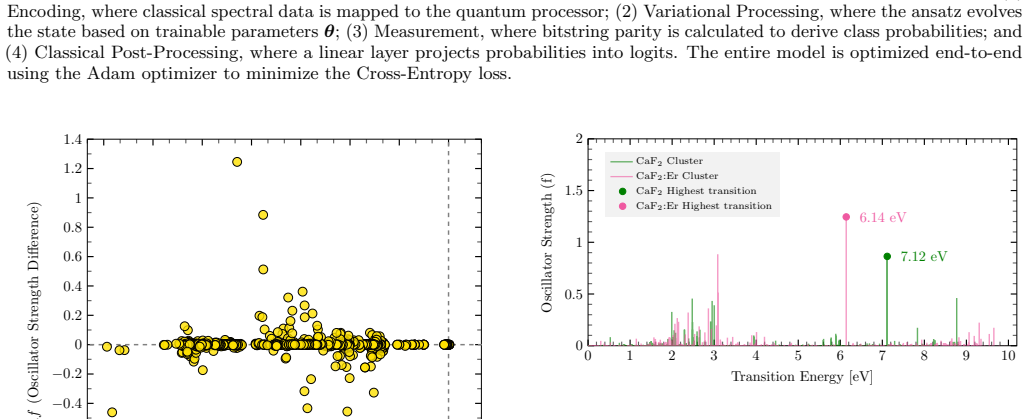
The core claim is that dopant-induced changes in the absorption spectrum are a sufficient and physically meaningful signature for classification. Replacing one calcium atom with erbium in a Ca8F16 cluster systematically red-shifts the dominant optical transitions and redistributes oscillator strength, producing enhanced visible absorption near 3 eV and shifting the strongest UV transition from about 7.1 to 6.1 eV. Once the discrete transitions are broadened into continuous spectra, the absorption coefficient, extinction coefficient, and transition energy separate the two systems almost perfectly in a classical kernel model. The same three descriptors, embedded through a quantum feature map,
Load-bearing premise
The load-bearing premise is that the 1,589 energy-resolved points per system are independent, exchangeable samples, even though they are densely spaced points along two smooth absorption curves, so the reported accuracies measure generalization rather than interpolation of the two known spectra.
Editorial extensions
If this is right
- The three selected descriptors carry almost all discriminative information: a classical RBF-kernel SVM achieves 0.983 test accuracy and 0.999 ROC-AUC.
- Fixed quantum kernels underperform the classical baseline: 0.851 accuracy on an ideal simulator, 0.817 under simulated depolarizing noise, and 0.733 on real quantum hardware.
- A trainable hybrid quantum neural network reaches 0.93 test accuracy and 0.96 AUC, improving on fixed quantum kernels but still below the classical SVM.
- The distinguishing spectral features persist across Gaussian broadening widths from 0.1 to 0.2 eV, indicating the fingerprint is not an artifact of the broadening choice.
- The end-to-end pipeline—from first-principles spectra to feature selection to quantum kernel execution on hardware—runs successfully and stays above random guessing, even under finite-shot and decoherence constraints.
Reading between the lines
- Because the 1,589 energy points per system are densely sampled along two smooth absorption curves, random point-wise train/test splits likely let classifiers interpolate the two known spectra; a harder and more meaningful benchmark would use independent material instances, such as different dopant concentrations, host sizes, or configurations.
- The same three descriptors could be tested for transfer to other rare-earth dopants or fluoride hosts; strong transfer would show the fingerprints are dopant-generic, while collapse would reveal that they are specific to the CaF2:Er pair studied here.
- The hardware-versus-simulation gap (0.733 vs 0.851) suggests a concrete follow-up test: increasing shot counts or applying error mitigation should move hardware accuracy toward the noisy-simulator value, a prediction that follows from the paper's own noise explanation but is not tested there.
- If the aim is to benchmark near-term quantum learning, labeling individual energy bins on two known spectra is easier than classifying unseen material instances; future work should separate these two tasks explicitly.
Editorial analysis
A structured set of objections, weighed in public.
Referee Report
Summary. The paper constructs finite clusters of pristine CaF2 (Ca8F16) and Er-doped CaF2 (Ca7ErF16), computes their optical spectra with LR-TDDFT, and derives energy-resolved descriptors (transition energy E, extinction coefficient κ, absorption coefficient α) at 1,589 points per system. These descriptors are fed into a classical RBF SVM, quantum SVMs (statevector, noisy QASM, IBM hardware), and a hybrid quantum neural network. The reported accuracies are 0.983 (classical SVM), 0.851/0.817 (QSVM simulators), 0.733 (hardware QSVM on a 15-sample test slice), and 0.93 (hybrid QNN). The paper claims these results establish a robust, physically grounded feature space for benchmarking near-term quantum learning models against classical baselines.
Significance. If the benchmark were valid, the work would provide a useful template for combining first-principles optical descriptors with quantum classifiers, and the comparison of classical, simulator, and hardware results would inform NISQ-era materials informatics. The TDDFT workflow, including cluster construction, Casida calculations, and Gaussian broadening, is described in sufficient detail to be reproduced, and the authors provide code and data. However, the central statistical claim is undermined by the data construction: the 1,589 samples per class are not independent measurements but densely sampled points along two smooth, deterministic absorption curves. Consequently, the high classification accuracies largely reflect interpolation of two known spectra rather than generalization to new materials, dopant concentrations, or noise levels. This invalidates the abstract's claim that the feature space is 'robust' and that the benchmarks are meaningful. The paper's internal caveats (§III.E: the hardware slice 'cannot be considered definitive'; §II.B: the descriptor set is 'a set instead of an unordered sequence') do not address this more fundamental limitation.
major comments (3)
- [§II.A, §III.B, Table I, Figure 8] The dataset consists of 1,589 energy-resolved points from each of only two smooth absorption spectra, one per material. Under the random point-wise train/test split used in §III.B–C, test points lie at energies immediately adjacent to training points on the same curve. Because the descriptors E, κ, α are continuous functions of energy with correlation length set by the Gaussian broadening σ=0.1–0.2 eV (Eq. 4) and the sampling spacing is much finer, the classifiers interpolate two known spectra. The reported test accuracy (0.983), AUC (0.999), and QML accuracies therefore do not measure generalization to unseen materials or configurations; they measure separability of two curves. The manuscript nowhere treats the two spectra as the evaluation unit. This is the load-bearing issue for the central claim that the descriptors form a 'robust feature space.'
- [§III.C–D, bootstrap confidence intervals] The bootstrap confidence intervals (e.g., classical SVM mean 0.983, 95% CI [0.965, 0.997]; QSVM SV [0.810, 0.893]) resample from the same dependent point dataset. Since the points are autocorrelated along each spectrum, the bootstrap only reflects sampling variability among correlated points on two fixed curves, not between-spectrum variability. It provides no evidence about how the models would perform on other dopant concentrations, cluster sizes, or disorder realizations. This does not rescue the generalization claim.
- [Abstract, §III.C, §III.F] The conclusion that dopant-induced optical fingerprints form a 'robust, physically grounded feature space for benchmarking near-term quantum learning models against strong classical baselines' is not supported by the experimental design. With only two systems, any sufficiently flexible classifier can achieve near-perfect separation on a fine energy grid. The physical descriptors may indeed be informative, but the benchmark as constructed cannot validate that claim. Demonstrating robustness would require multiple doped/undoped instances (different concentrations, cluster sizes, or host variants) with evaluation at the spectrum level, not at the level of individual energy points.
minor comments (4)
- [§III.E] The hardware QSVM uses only 30 training and 15 test samples; the authors correctly note that these results 'cannot be considered definitive,' but the small sample size should be more prominently featured in the abstract and conclusion, where the hardware accuracy is reported without qualification.
- [§II.B and Figure 9] Feature selection via linear SVM weights is performed on the data before describing the train/test split. If the weight-based ranking uses all 3,178 points, the selected features (α, κ, E) may incorporate information from the test set. The authors should clarify whether feature selection was nested inside the training folds or performed on the full dataset.
- [General] Some notation is introduced without explicit definition (e.g., 'N_{occ}' in Eq. 1, 'E_min' in Eq. 21). The paper would benefit from a table summarizing all hyperparameters and dataset sizes for each model, including the QNN's effective training sample count of 2,304 points and the relationship between this number and the 1,589-point per-system dataset.
- [§IV and Table II] The discussion compares QSVM and QNN accuracies across heterogeneous datasets (MNIST, hyperspectral images, polymer band gaps, ADME-Tox). These comparisons are not quantitatively meaningful without controlling for task difficulty, data size, and evaluation protocol. The text should clearly state that cross-dataset accuracy comparisons are illustrative only.
Circularity Check
No significant circularity: the classification benchmark uses simulated spectra and labels set by cluster composition, not by fitted outputs of the model itself.
full rationale
The paper's derivation chain is linear: DFT/TDDFT calculations (Eqs. 1-4) produce optical spectra, from which descriptors (E, kappa, alpha) are extracted; those descriptors are then fed into classical and quantum classifiers (Eqs. 6-21), and test accuracies are reported. Nowhere does a fitted parameter or a predicted quantity feed back into the definition of the descriptors or the labels. The class labels (pristine vs. Er-doped) are fixed by the cluster construction before any calculation, so the high classification accuracy is not obtained by fitting something and then re-predicting the same fitted quantity. The point-wise train/test split does mean that test points are interleaved with training points along two smooth spectra, so the reported accuracies partly reflect interpolation rather than generalization to new materials; that is a legitimate statistical/benchmark-validity concern, but it is not circularity under the definitions used here. The self-citations (e.g., refs. [3], [8], [13]) are contextual and not load-bearing for the main derivation. The paper itself explicitly cautions that the small hardware slice 'cannot be considered definitive' (§III.E), which further shows the authors do not overstate that result. Overall, the central claim is an empirical demonstration of separability of known spectra, not a derivation that reduces to its inputs.
Assumptions & free parameters
free parameters (4)
- Gaussian broadening width σ =
0.1–0.2 eV
- Box-Cox transformation λ per feature =
estimated from training data
- Energy grid sampling =
1,589 points over 0–10 eV
- QNN hyperparameters =
L=4 ansatz depth, d=1 feature-map repetition, learning-rate scheduler, early-stopping patience
assumptions (4)
- domain assumption PBE DFT and LR-TDDFT (Casida) give a faithful description of the relative optical spectra of CaF2 and CaF2:Er.
- domain assumption A 24-atom cluster with 6–10 Å vacuum represents the bulk fluorite and the dilute doping limit.
- domain assumption Each of the 1,589 energy points per system is an independent sample for ML training and testing.
- domain assumption The selected descriptors α, κ, E constitute a sufficient representation for the classification task.
Cite this review
Pith. "Pith review of First-Principles Optical Descriptors and Hybrid Classical-Quantum Classification of Er-Doped CaF$_2$." pith.science (2026). https://pith.science/paper/BCXXYM2Z
@misc{pith2026260200525,
  author       = {Pith},
  title        = {Pith review of: First-Principles Optical Descriptors and Hybrid Classical-Quantum Classification of Er-Doped CaF$_2$},
  year         = {2026},
  howpublished = {\url{https://pith.science/paper/BCXXYM2Z}},
  note         = {Machine review of arXiv:2602.00525}
}
abstract
We present a physics-informed classical-quantum machine learning framework for discriminating pristine CaF$_2$ from Er-doped CaF$_2$ using first-principles optical descriptors. Finite Ca$_8$F$_{16}$ and Ca$_7$ErF$_{16}$ clusters were constructed from the fluorite structure (a=5.46~$\AA$) and treated using density functional theory (DFT) and linear-response time-dependent DFT (LR-TDDFT) within the GPAW code. Geometry optimization was performed in LCAO mode with a DZP basis and PBE exchange-correlation functional, followed by real-space finite-difference ground-state calculations with grid spacing h=0.30~$\AA$ and N$_{bands}$=N$_{occ}$+20. Optical excitations up to 10~eV were obtained via the Casida formalism and converted into continuous absorption spectra using Gaussian broadening ($\sigma$=0.1-0.2~eV). From 1,589 energy-resolved points per system, physically interpretable descriptors including transition energy $E$, extinction coefficient $\kappa$, and absorption coefficient $\alpha$ were extracted. A classical RBF-kernel support vector machine (SVM) achieves a test accuracy (ACC) of 0.983 and ROC-AUC of 0.999. Quantum support vector machines (QSVMs) evaluated on statevector and noisy simulators reach accuracies of 0.851 and 0.817, respectively, while execution on IBM quantum hardware yields a test-slice accuracy of 0.733 under finite-shot and decoherence constraints. A hybrid quantum neural network (QNN) with a 3-qubit feature map and depth-4 ansatz achieves a test accuracy of 0.93 and AUC of 0.96. Results here demonstrate that dopant-induced optical fingerprints form a robust, physically grounded feature space for benchmarking near-term quantum learning models against strong classical baselines.
Figures


Figures from the paper (11 more)




Reference graph
Works this paper leans on
-
[1]
Auzel, Chemical reviews104, 139 (2004)
F. Auzel, Chemical reviews104, 139 (2004)
2004
-
[2]
R. W. Boyd, A. L. Gaeta, and E. Giese, inSpringer Hand- book of Atomic, Molecular, and Optical Physics(Springer,
-
[3]
D. D. K. Wayo, M. Z. B. M. Noor, M. D. Ganji, and L. Goliatt, Luminescence40, e70297 (2025)
2025
-
[4]
Haase and H
M. Haase and H. Sch¨ afer, Angewandte Chemie Interna- tional Edition50, 5808 (2011)
2011
-
[5]
B. Zhou, B. Shi, D. Jin, and X. Liu, Nature nanotechnol- ogy10, 924 (2015)
2015
-
[6]
G. Chen, H. ˚Agren, T. Y. Ohulchanskyy, and P. N. Prasad, Chemical Society Reviews44, 1680 (2015)
2015
-
[7]
Wang and X
F. Wang and X. Liu, Chemical Society Reviews38, 976 (2009)
2009
-
[8]
D. D. K. Wayo, L. Goliatt, and M. D. Ganji, Reviews in Chemical Engineering41, 741 (2025)
2025
Show all 56 references
-
[9]
D. S. Sholl and J. A. Steckel,Density functional theory: a practical introduction(John Wiley & Sons, 2022)
2022
-
[10]
M. A. Marques, N. T. Maitra, F. M. Nogueira, E. K. Gross, and A. Rubio,Fundamentals of time-dependent density functional theory, Vol. 837 (Springer, 2012)
2012
-
[11]
K. T. Butler, D. W. Davies, H. Cartwright, O. Isayev, and A. Walsh, Nature559, 547 (2018)
2018
-
[12]
Schmidt, M
J. Schmidt, M. R. Marques, S. Botti, and M. A. Marques, npj computational materials5, 83 (2019)
2019
-
[13]
D. D. K. Wayo, Archives of Computational Methods in Engineering , 1 (2025)
2025
-
[14]
Raccuglia, K
P. Raccuglia, K. C. Elbert, P. D. Adler, C. Falk, M. B. Wenny, A. Mollo, M. Zeller, S. A. Friedler, J. Schrier, and A. J. Norquist, Nature533, 73 (2016)
2016
-
[15]
Biamonte, P
J. Biamonte, P. Wittek, N. Pancotti, P. Rebentrost, N. Wiebe, and S. Lloyd, Nature549, 195 (2017)
2017
-
[16]
Schuld and N
M. Schuld and N. Killoran, Prx Quantum3, 030101 (2022)
2022
-
[17]
Enkovaara, C
J. Enkovaara, C. Rostgaard, J. J. Mortensen, J. Chen, M. Du lak, L. Ferrighi, J. Gavnholt, C. Glinsvad, V. Haikola, H. A. Hansen,et al., Journal of physics: Con- densed matter22, 253202 (2010)
2010
-
[18]
J. J. Mortensen, L. B. Hansen, and K. W. Jacobsen, Physical Review B—Condensed Matter and Materials Physics71, 035109 (2005)
2005
-
[19]
A. H. Larsen, J. J. Mortensen, J. Blomqvist, I. E. Castelli, R. Christensen, M. Du lak, J. Friis, M. N. Groves, B. Ham- mer, C. Hargus,et al., Journal of Physics: Condensed Matter29, 273002 (2017)
2017
-
[20]
O’Keeffe and B
M. O’Keeffe and B. G. Hyde,Crystal structures(Courier Dover Publications, 2020)
2020
-
[21]
H. W. Moos, Journal of Luminescence1, 106 (1970)
1970
-
[22]
Reisfeld, inHalide Glasses for Infrared Fiberoptics (Springer, 1987) pp
R. Reisfeld, inHalide Glasses for Infrared Fiberoptics (Springer, 1987) pp. 237–252. 16
1987
-
[23]
J. P. Perdew, K. Burke, and M. Ernzerhof, Physical review letters77, 3865 (1996)
1996
-
[24]
M. E. Casida, inRecent Advances In Density Functional Methods: (Part I)(World Scientific, 1995) pp. 155–192
1995
-
[25]
Onida, L
G. Onida, L. Reining, and A. Rubio, Reviews of modern physics74, 601 (2002)
2002
-
[26]
G. E. P. Box and D. R. Cox, Journal of the Royal Statis- tical Society: Series B (Methodological)26, 211 (2018)
2018
-
[27]
Cortes and V
C. Cortes and V. Vapnik, Machine Learning20, 273 (1995)
1995
-
[28]
Chang and C.-J
C.-C. Chang and C.-J. Lin, ACM transactions on intelli- gent systems and technology (TIST)2, 1 (2011)
2011
-
[29]
Rebentrost, M
P. Rebentrost, M. Mohseni, and S. Lloyd, Phys. Rev. Lett. 113, 130503 (2014)
2014
-
[30]
Havl ´ ıˇ cek, A
V. Havl ´ ıˇ cek, A. D. C´ orcoles, K. Temme, A. W. Harrow, A. Kandala, J. M. Chow, and J. M. Gambetta, Nature 567, 209–212 (2019)
2019
-
[31]
Cerezo, A
M. Cerezo, A. Arrasmith, R. Babbush, S. C. Benjamin, S. Endo, K. Fujii, J. R. McClean, K. Mitarai, X. Yuan, L. Cincio, and P. J. Coles, Nature Reviews Physics3, 625–644 (2021)
2021
-
[32]
Benedetti, E
M. Benedetti, E. Lloyd, S. Sack, and M. Fiorentini, Quan- tum Science and Technology4, 043001 (2019)
2019
-
[33]
S. Sim, P. D. Johnson, and A. Aspuru-Guzik, Advanced Quantum Technologies2, 10.1002/qute.201900070 (2019)
2019 doi
-
[34]
Schuld, V
M. Schuld, V. Bergholm, C. Gogolin, J. Izaac, and N. Kil- loran, Physical Review A99, 032331 (2019)
2019
- [35]
-
[36]
Goodfellow, Y
I. Goodfellow, Y. Bengio, and A. Courville,Deep Learning (MIT Press, 2016)
2016
-
[37]
D. P. Kingma and J. Ba, arXiv preprint arXiv:1412.6980 (2014)
2014 arXiv
-
[38]
S. J. Reddi, S. Kale, and S. Kumar, inInternational Conference on Learning Representations(2018)
2018
-
[39]
Bengio, inNeural networks: Tricks of the trade (Springer, 2012) pp
Y. Bengio, inNeural networks: Tricks of the trade (Springer, 2012) pp. 437–478
2012
-
[40]
Prechelt, inNeural Networks: Tricks of the Trade (Springer, 1998) pp
L. Prechelt, inNeural Networks: Tricks of the Trade (Springer, 1998) pp. 55–69
1998
-
[41]
J. R. McClean, S. Boixo, V. N. Smelyanskiy, R. Babbush, and H. Neven, Nature Communications9, 10.1038/s41467- 018-07090-4 (2018)
2018 doi
-
[42]
A. C. Doner, H. A. Moran, A. R. Webb, M. G. Christian- son, A. L. Koritzke, N. S. Dewey, S. W. Hartness, and B. Rotavera, Journal of Quantitative Spectroscopy and Radiative Transfer297, 108438 (2023)
2023
-
[43]
A. G. Pai, K. M. Buddhiraju, and S. S. Durbha, inRe- mote Sensing for Agriculture, Ecosystems, and Hydrology XXIV, Vol. 12262, edited by C. M. U. Neale and A. Mal- tese, International Society for Optics and Photonics (SPIE,
-
[44]
Stoyanova, T
A. Stoyanova, T. Hammadia, A. Ricou, and B. Penkovsky, Photonic quantum computing for polymer classification (2022), arXiv:2211.12207 [quant-ph]
2022 arXiv
-
[45]
A. S. Bhatia, M. K. Saggi, and S. Kais, Journal of Chem- ical Information and Modeling63, 6476 (2023), pMID: 37603536
2023
-
[46]
Hirai, arXiv preprint arXiv:2310.17935 (2023)
H. Hirai, arXiv preprint arXiv:2310.17935 (2023)
2023 arXiv
-
[47]
Juno Ryu, E
E. Juno Ryu, E. Abo, and K. June-Koo, Materials (2023)
2023
-
[48]
C. Long, M. Huang, X. Ye, Y. Futamura, and T. Sakurai, Scientific Reports15, 31780 (2025)
2025
-
[49]
J. Wu, Z. Tao, and Q. Li, in2022 IEEE International Con- ference on Quantum Computing and Engineering (QCE) (IEEE, 2022) pp. 38–48
2022
-
[50]
Rodriguez-Grasa, Y
P. Rodriguez-Grasa, Y. Ban, and M. Sanz, Physical Re- view Research7, 023269 (2025)
2025
-
[51]
Xia and S
R. Xia and S. Kais, Entropy22, 828 (2020)
2020
-
[52]
Correll, S
R. Correll, S. J. Weinberg, F. Sanches, T. Ide, and T. Suzuki, Advanced Quantum Technologies6, 2200183 (2023)
2023
-
[53]
L. C. Sander, N. A. McMahon, P. Zapletal, and M. J. Hartmann, Physical Review Research7, L042032 (2025)
2025
-
[54]
Gupta, D
S. Gupta, D. Konar, and V. Aggarwal, A scalable quantum non-local neural network for image classification (2024), arXiv:2407.18906
2024 arXiv
-
[55]
Tacchino, C
F. Tacchino, C. Macchiavello, D. Gerace, and D. Bajoni, npj Quantum Information5, 1 (2019)
2019
-
[56]
M. E. Sahin, E. Altamura, O. Wallis, S. P. Wood, A. Dekusar, D. A. Millar, T. Imamichi, A. Matsuo, and S. Mensa, arXiv preprint arXiv:2505.17756 (2025)
2025 arXiv
Reviewed August 3, 2026 · model on record in the stance chip above.
Discussion (0). Continue with ORCID to comment.