REVIEW 3 major objections 5 minor 60 references
Likelihood-Free Variational Autoencoders
T0 review · 3 major / 5 minor · reviewed 2026-08-16 · deepseek-v4-flash
Pith's one-line read This paper proposes replacing a VAE's Gaussian likelihood with the energy score, a strictly proper scoring rule, and shows that the resulting likelihood-free EnVAE and its single-sample variant FEnVAE improve image reconstruction and…
desk verdict The single-sample surrogate is a genuinely useful trick, but the paper's central propriety argument is misapplied and needs serious reworking before the 'statistically principled' claim can be taken literally. read the letter →
The pith
A machine-rendered reading of the paper's core claim, the machinery that carries it, and where it could break.
The reading
What carries the argument
The central object is the energy score, a strictly proper scoring rule defined as $$S_E(P,x) = \mathbb{E}_{X\sim P}\|X-x\|_2^\$\beta$ - \tfrac{1}{2}\mathbb{E}_{X,X'\sim P}\|X-X'\|_2^\$\beta$,$$ whose expected value is uniquely minimized when the predicted distribution $P$ equals the true data distribution. In EnVAE, $P$ is the distribution of decoded outputs $g_\theta(z)$ with $z \sim q_\phi(z|x)$, so the score becomes a sample-based reconstruction loss. The key simplification in FEnVAE is a first-order Taylor expansion of the decoder, $g_\theta(z) \approx g_\theta(\mu_z) + J_{\mu_z}(z-\mu_z)$, which rewrites the pairwise dispersion term using the latent covariance and then re-expresses it through decoder outputs alone. That yields the single-sample objective $$L^*(\$\theta$,\phi;x) = \|g_\$\theta$(z^*) - x\|_2^\$\beta$ - \tfrac{1}{2}\|g_\$\theta$(\mu_z + \sqrt{2}(z^*-\mu_z)) - g_\$\theta$(\mu_z)\|_2^\$\beta$ + \$\alpha$ D_{\mathrm{KL}}(q_\$\varphi$(z|x)\|p(z)).$$
What would settle it
Train EnVAE on synthetic data drawn from a known nonlinear decoder with substantial latent variance, then test the learned sampler against the true data distribution with a two-sample energy-distance test; if the test rejects at the paper's sample sizes, the propriety-based claim fails. Separately, if FEnVAE's single-sample loss diverges from EnVAE's multi-sample loss as latent variance grows or decoder curvature increases, the local-linearity premise is falsified.
Extended reading notes
Core claim
The paper's central claim is that VAEs can be trained without any parametric likelihood by pairing a deterministic decoder with the energy score as the reconstruction objective. For an input $x$, the encoder produces a Gaussian posterior over latent $z$, samples are decoded, and the loss is the expected distance from decoded samples to $x$ minus half the expected pairwise distance among decoded samples, plus the usual KL regularizer toward the prior. Because the energy score is strictly proper, the paper argues that minimizing it favors the correct output distribution in expectation; because the decoder is deterministic, no density for $p_\theta(x|z)$ is ever evaluated. The fast variant FEnVAE replaces the pairwise Monte Carlo term with a closed-form surrogate built from a first-order Taylor expansion of the decoder around the posterior mean, reusing a single noise draw in both the mean and dispersion terms. Empirically, EnVAE and FEnVAE improve FID for reconstruction and generation over Gaussian, Laplace, Student-t, and frequency-based baselines on CelebA 64, CIFAR-10, and LSUN Church.
Load-bearing premise
The paper's argument stands on the assumption that scoring an encoder's conditional output distribution with the energy score pushes the model's overall output distribution toward the true data distribution, a step the paper asserts but does not prove; FEnVAE additionally assumes the decoder is nearly linear over the small spread of latent samples.
Editorial extensions
If this is right
- VAE pipelines can retain amortized inference and latent-space regularization while dropping the likelihood model; the same architecture can be trained with a scoring-rule loss at minimal added cost.
- The single-sample FEnVAE objective makes the energy score practical at scale, with overhead of roughly two extra decoder passes, so large VAE-based systems could adopt likelihood-free reconstruction without architectural changes.
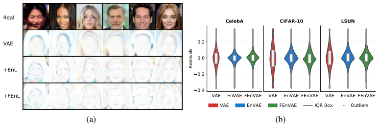
- Reconstruction uncertainty is represented by the spread of decoded samples rather than by a parameterized noise model, which yields sharper pixel-wise variance maps in the paper's visualizations.
- Because the loss is a proper score rather than an adversarial objective, training remains stable and no discriminator is needed, potentially capturing some GAN-like sharpness without GAN training dynamics.
- The score's $\beta$ exponent controls sensitivity to large errors; the paper shows $\beta=1$ works best and $\beta=2$ degenerates to MSE, so $\beta$ becomes a practical tuning knob connecting the method to standard losses.
Reading between the lines
- If the propriety transfer holds in the autoencoder conditional setting, the same construction could replace likelihood terms in other latent-variable models, such as hierarchical VAEs, normalizing-flow decoders, or time-series forecasting models, not just image autoencoders.
- The FEnVAE approximation should degrade as posterior variance grows or decoder curvature increases; the paper's own tables show larger latent variance correlating with larger FEnVAE-vs-EnVAE gaps, suggesting a testable bound relating approximation error to the latent covariance and the Jacobian's Lipschitz constant.
- A deeper consequence is that blur in VAEs may be attributed less to the KL term itself and more to the Gaussian observation model; if so, likelihood-free reconstruction could be combined with more aggressive latent regularization to trade off sharpness and coverage.
Signed reviews
Editorial analysis
A structured set of objections, weighed in public.
Referee Report
Summary. The paper proposes EnVAE, a VAE variant with a deterministic decoder g_theta trained by minimizing the energy score between the conditional predictive distribution q_phi(z|x) decoded through g_theta and the observation x, plus a KL regularizer. It also introduces FEnVAE, a single-sample surrogate obtained from a first-order Taylor expansion of the decoder, in which the pairwise dispersion term is replaced by a finite-difference term evaluated at one perturbed latent sample. Experiments on CelebA, CIFAR-10, and LSUN report lower FID for reconstruction and generation than likelihood-based reconstruction losses, and consistent gains when the loss is plugged into several existing VAE baselines. The authors claim that proper scoring-rule theory makes the approach statistically principled.
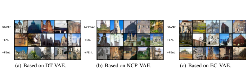
Significance. If the theoretical framing were valid, the paper would offer an interesting bridge between proper scoring rules and amortized variational inference. The empirical work is a strength: it covers multiple datasets and baselines, integrates the loss into three existing VAE/EBM models, includes efficiency and ablation analyses, and provides a public code repository. However, the central statistical claim is not established. The propriety of the energy score is invoked for a conditional reconstruction distribution whose target is the conditioning observation itself; this does not imply that the marginal generated distribution matches the data. The FEnVAE derivation also contains an unjustified replacement of a Jacobian term by a nonlinear finite difference, and the reported smoothness validation measures the encoder rather than the decoder. As a result, the paper currently reads as an empirical demonstration of an energy-score-inspired reconstruction loss rather than as a principled likelihood-free VAE.
major comments (3)
- [3.1, Eq. (4)] The propriety of the energy score is transferred from standard scoring-rule theory to an autoencoder objective without justification. In Gneiting and Raftery (2007), a proper scoring rule S(Q,y) is minimized in expectation over y~P by Q=P for a fixed predictive distribution Q. In Eq. (4), the predictive distribution Q_{theta,phi}(x) is constructed by an encoder that receives x itself, and the population objective is E_{x~p_data}[S(Q_{theta,phi}(x),x)]. For each x, the optimal conditional predictive distribution is the degenerate measure delta_x, so minimizing this score enforces pointwise reconstruction and does not, by itself, constrain the marginal generator g_theta#p(z). The statements in Section 3.1 ("we aim to learn a generative model that accurately reflects the underlying data distribution") and Appendix 6.1.3 ("the score's propriety ensures that, in expectation, the correct data distribution is favored") therefore do not follow from propriety. The paper needs either a proof that the combination with the KL term yields marginal matching, or a careful restatement of the theoretical claims.
- [3.2, Eqs. (11)-(13)] The derivation of the FEnVAE objective replaces the term ||J_{mu_z} Sigma_z^{1/2} ehat||^beta in Eq. (11) with ||g_theta(mu_z+Sigma_z^{1/2} ehat)-g_theta(mu_z)||^beta using Eq. (12). But Eq. (12) is itself the first-order Taylor approximation of the decoder. For a nonlinear decoder, the finite-difference term is not equal to the Jacobian term, and the claim that this replacement "locally restores the nonlinear modeling capability" is not supported. The final loss in Eq. (14) is therefore a new heuristic surrogate rather than a closed-form evaluation of the energy score under the stated linearity assumption. The paper should state the approximation being made at this step and justify why the finite-difference replacement is preferable to retaining the Jacobian term.
- [4.3.2, Appendix 6.5, Eq. (26)] The empirical validation of the local-linearity assumption uses the Lipschitz constant of the encoder f(x), but the Taylor expansion in Section 3.2 is taken with respect to the decoder g_theta(z). The smoothness of the encoder does not directly control the size of the omitted O(||z-mu_z||^2) term in Eq. (8), so the Lip values reported in Tables 3-4 and the surrounding discussion do not validate the assumption that underlies FEnVAE. The paper should either measure a relevant decoder Jacobian or Hessian quantity, or reformulate the validity check to target the decoder.
minor comments (5)
- [Eq. (3)] The summation limits in the second term of Eq. (3) are garbled: the text reads "sum_{i=j} sum_{j:j neq i}", which should presumably be "sum_{i=1}^M sum_{j:j neq i}". Please correct this typo.
- [Appendix 6.3, Eq. (18)] The finite-M calculation for beta=2 is algebraically inconsistent. The pairwise sum in Eq. (3) evaluates to - (1/(M-1)) sum_i ||x_i - x_mu||^2 with the usual unbiased variance convention, not the expression used in Eq. (18). The conclusion that beta=2 reduces to the squared Euclidean distance is correct in the population limit, but the displayed derivation should be repaired.
- [Figures 1-3] The figure numbering is confusing and duplicated: Figures 1-3 in Section 3.2 are methodology diagrams, while Figures 2-3 in Section 4 are reconstruction and generation samples. Please renumber all figures and ensure each caption matches its content.
- [Eq. (14)] The KL term in Eq. (14) is written as D_KL(q_phi(z|x) || p_theta(z)), but the prior elsewhere in the paper is denoted p(z) and is not parameterized by theta. Please make the notation consistent.
- [6.13] The text says "beta is the exponent of the frequency domain energy score," but the energy score in Eq. (1) is defined in the data domain. The frequency-domain interpretation appears only in the qualitative discussion of spectral plots and should be stated as an interpretation rather than a definition.
Circularity Check
The 'statistically principled' claim reduces to per-example reconstruction: the energy score is scored against the same conditioning point, so by construction the correct predictive distribution is δ_x, not the marginal data distribution.
-
self definitional
[Section 3.1, paragraph after Eq. (3); echoed in Appendix 6.1.3]
"By minimizing the energy score, we aim to learn a generative model that accurately reflects the underlying data distribution."
In the definition of a proper scoring rule, the expectation of S(P,Y) is minimized over predictive distributions P when P equals the law of the observed outcome Y. In Eq. (2) the 'predicted distribution' is Q_{θ,φ}(x)=g_θ#q_φ(·|x), and the observed outcome scored is the very same x that conditions the encoder. The population objective is thus E_{x~p_data}[S(Q(x),x)], and for each fixed x the score is minimized by Q(x)=δ_x by construction. This forces per-example reconstruction but does not by itself compare the sampling distribution g_θ#p(z) with p_data; the KL term only pulls q(z|x) toward the prior.
full rationale
The paper's empirical contribution is not circular: EnVAE and FEnVAE are evaluated against external benchmarks and baselines, the FEnVAE loss in Eq. (14) follows from a Taylor expansion with no constants fitted to the reported FID values, and the β=2 degeneration to MSE is acknowledged rather than hidden. There is no load-bearing self-citation chain or imported uniqueness theorem. However, the central theoretical justification that minimizing the energy score 'accurately reflects the underlying data distribution' is circular in a narrower sense: the scoring pair used in Eq. (2) is (x,x), where the same data point acts as both the conditioning input to the encoder and the observed outcome of the predictive distribution. In that pair the 'true data distribution' is δ_x by construction, so propriety enforces reconstruction fidelity and cannot by itself justify matching the marginal generator g_θ#p(z) to p_data. The score is thus proportional to the strength of the reconstruction objective, not an independently derived guarantee of generative fidelity. The rest of the derivations are self-contained, so the overall circularity is partial rather than total.
Assumptions & free parameters
free parameters (3)
- beta (energy score exponent) =
1 (chosen via hyperparameter sweep in Fig. 24)
- alpha (KL weight) =
not reported in main text
- M (number of Monte Carlo samples for EnVAE) =
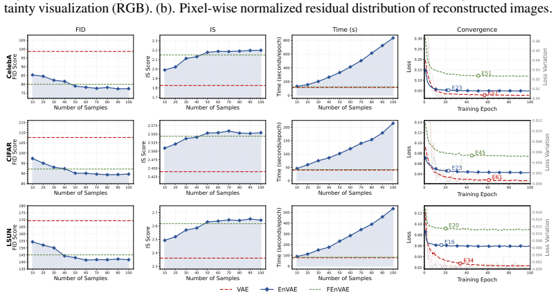
up to 100 in experiments; reported performance plateaus near 50-100
assumptions (5)
- standard math The energy score is a strictly proper scoring rule
- domain assumption First-order Taylor expansion of the decoder is valid near the posterior mean
- domain assumption Minimizing the per-example reconstruction energy score plus KL aligns the model's marginal generative distribution with the data
- standard math Single-sample shared-noise estimator approximates the expectation of the energy score
- domain assumption Standard normal prior and diagonal Gaussian posterior
Cite this review
Pith. "Pith review of Likelihood-Free Variational Autoencoders." pith.science (2026). https://pith.science/paper/BGD7364V
@misc{pith2026250417622,
  author       = {Pith},
  title        = {Pith review of: Likelihood-Free Variational Autoencoders},
  year         = {2026},
  howpublished = {\url{https://pith.science/paper/BGD7364V}},
  note         = {Machine review of arXiv:2504.17622}
}
read the original abstract
Variational Autoencoders (VAEs) typically rely on a probabilistic decoder with a predefined likelihood, most commonly an isotropic Gaussian, to model the data conditional on latent variables. While convenient for optimization, this choice often leads to likelihood misspecification, resulting in blurry reconstructions and poor data fidelity, especially for high-dimensional data such as images. In this work, we propose EnVAE, a novel likelihood-free generative framework that has a deterministic decoder and employs the energy score--a proper scoring rule--to build the reconstruction loss. This enables likelihood-free inference without requiring explicit parametric density functions. To address the computational inefficiency of the energy score, we introduce a fast variant, FEnVAE, based on the local smoothness of the decoder and the sharpness of the posterior distribution of latent variables. This yields an efficient single-sample training objective that integrates seamlessly into existing VAE pipelines with minimal overhead. Empirical results on standard benchmarks demonstrate that EnVAE achieves superior reconstruction and generation quality compared to likelihood-based baselines. Our framework offers a general, scalable, and statistically principled alternative for flexible and nonparametric distribution learning in generative modeling.
Figures


Figures from the paper (23 more)




Reference graph
Works this paper leans on
-
[1]
Auto-encoding variational bayes,
D. P. Kingma and M. Welling, “Auto-encoding variational bayes,” inInternational Conference on Learning Representations, 2014
work page 2014
-
[2]
I. Goodfellow, J. Pouget-Abadie, M. Mirza, B. Xu, D. Warde-Farley, S. Ozair, A. Courville, and Y . Bengio, “Generative adversarial nets,”Advances in Neural Information Processing Sys- tems, vol. 27, 2014
work page 2014
-
[3]
Variational inference with normalizing flows,
D. Rezende and S. Mohamed, “Variational inference with normalizing flows,” in International Conference on Machine Learning, 2015, pp. 1530–1538
work page 2015
-
[4]
Make a face: To- wards arbitrary high fidelity face manipulation,
S. Qian, K.-Y . Lin, W. Wu, Y . Liu, Q. Wang, F. Shen, C. Qian, and R. He, “Make a face: To- wards arbitrary high fidelity face manipulation,” inProceedings of the IEEE/CVF International Conference on Computer Cision, 2019, pp. 10 033–10 042
work page 2019
-
[5]
Introvae: Introspective variational autoencoders for photographic image synthesis,
H. Huang, R. He, Z. Sun, T. Tan et al., “Introvae: Introspective variational autoencoders for photographic image synthesis,” Advances in Neural Information Processing Systems, vol. 31, 2018
work page 2018
-
[6]
Conditional variational autoencoder with adversarial learning for end-to-end text-to-speech,
J. Kim, J. Kong, and J. Son, “Conditional variational autoencoder with adversarial learning for end-to-end text-to-speech,” inInternational Conference on Machine Learning. PMLR, 2021, pp. 5530–5540
work page 2021
-
[7]
Portaspeech: Portable and high-quality generative text-to- speech,
Y . Ren, J. Liu, and Z. Zhao, “Portaspeech: Portable and high-quality generative text-to- speech,” Advances in Neural Information Processing Systems, vol. 34, 2021
work page 2021
-
[8]
Vector quantized diffusion model for text-to-image synthesis,
S. Gu, D. Chen, J. Bao, F. Wen, B. Zhang, D. Chen, L. Yuan, and B. Guo, “Vector quantized diffusion model for text-to-image synthesis,” in Proceedings of the IEEE/CVF Conference on Computer Vision and Pattern Recognition, 2022, pp. 10 696–10 706
2022
Show all 60 references
-
[9]
Causal recurrent variational autoencoder for medical time series generation,
H. Li, S. Yu, and J. Principe, “Causal recurrent variational autoencoder for medical time series generation,” in Proceedings of the AAAI Conference on Artificial Intelligence , vol. 37, no. 7, 2023, pp. 8562–8570
2023
-
[10]
Markovian gaussian process variational autoencoders,
H. Zhu, C. Balsells-Rodas, and Y . Li, “Markovian gaussian process variational autoencoders,” in International Conference on Machine Learning. PMLR, 2023, pp. 42 938–42 961
2023
-
[11]
beta-vae: Learning basic visual concepts with a constrained variational framework,
I. Higgins, L. Matthey, A. Pal, C. Burgess, X. Glorot, M. Botvinick, S. Mohamed, and A. Ler- chner, “beta-vae: Learning basic visual concepts with a constrained variational framework,” in International Conference on Learning Representations, 2017
2017
-
[12]
Isolating sources of disentanglement in variational autoencoders,
R. T. Chen, X. Li, R. B. Grosse, and D. K. Duvenaud, “Isolating sources of disentanglement in variational autoencoders,” Advances in Neural Information Processing Systems, vol. 31, 2018
2018
-
[13]
Distributional learning of variational autoencoder: application to syn- thetic data generation,
S. An and J.-J. Jeon, “Distributional learning of variational autoencoder: application to syn- thetic data generation,” Advances in Neural Information Processing Systems, vol. 36, 2024
2024
-
[14]
Explicitly minimizing the blur error of variational autoencoders,
G. Bredell, K. Flouris, K. Chaitanya, E. Erdil, and E. Konukoglu, “Explicitly minimizing the blur error of variational autoencoders,” in The Eleventh International Conference on Learning Representations, 2023. [Online]. Available: https://openreview.net/forum?id=9krnQ-ue9M
2023
-
[15]
An introduction to variational autoencoders,
D. P. Kingma and M. Welling, “An introduction to variational autoencoders,” Foundations and Trends® in Machine Learning , vol. 12, no. 4, pp. 307–392, 2019. [Online]. Available: http://dx.doi.org/10.1561/2200000056
2019 doi
-
[16]
Gaussian process prior varia- tional autoencoders,
F. P. Casale, A. Dalca, L. Saglietti, J. Listgarten, and N. Fusi, “Gaussian process prior varia- tional autoencoders,” Advances in Neural Information Processing Systems, vol. 31, 2018
2018
-
[17]
Structured uncertainty prediction networks,
G. Dorta, S. Vicente, L. Agapito, N. D. Campbell, and I. Simpson, “Structured uncertainty prediction networks,” in Proceedings of the IEEE Conference on Computer Vision and Pattern Recognition, 2018, pp. 5477–5485
2018
-
[18]
Variational laplace autoencoders,
Y . Park, C. Kim, and G. Kim, “Variational laplace autoencoders,” inInternational Conference on Machine Learning. PMLR, 2019, pp. 5032–5041
2019
-
[19]
Poisson variational autoencoder,
H. Vafaii, D. Galor, and J. Yates, “Poisson variational autoencoder,”Advances in Neural Infor- mation Processing Systems, vol. 37, 2024
2024
-
[20]
Variational autoencoders for sparse and overdispersed discrete data,
H. Zhao, P. Rai, L. Du, W. Buntine, D. Phung, and M. Zhou, “Variational autoencoders for sparse and overdispersed discrete data,” in International Conference on Artificial Intelligence and Statistics, 2020, pp. 1684–1694. 10
2020
-
[21]
Autoencoding variational inference for topic models,
A. Srivastava and C. Sutton, “Autoencoding variational inference for topic models,” arXiv preprint arXiv:1703.01488, 2017
2017 arXiv
-
[22]
t3-variational autoencoder: Learning heavy- tailed data with student’s t and power divergence,
J. Kim, J. Kwon, M. Cho, H. Lee, and J.-H. Won, “t3-variational autoencoder: Learning heavy- tailed data with student’s t and power divergence,” in International Conference on Learning Representations, 2024
2024
-
[23]
Student-t variational autoen- coder for robust density estimation
H. Takahashi, T. Iwata, Y . Yamanaka, M. Yamada, and S. Yagi, “Student-t variational autoen- coder for robust density estimation.” in IJCAI, 2018, pp. 2696–2702
2018
-
[24]
Nvae: A deep hierarchical variational autoencoder,
A. Vahdat and J. Kautz, “Nvae: A deep hierarchical variational autoencoder,” Advances in Neural Information Processing Systems, vol. 33, 2020
2020
-
[25]
Ladder variational autoencoders,
C. K. Sønderby, T. Raiko, L. Maaløe, S. K. Sønderby, and O. Winther, “Ladder variational autoencoders,” Advances in Neural Information Processing Systems, vol. 29, 2016
2016
-
[26]
Learning hierarchical features from generative models,
S. Zhao, J. Song, and S. Ermon, “Learning hierarchical features from generative models,” arXiv preprint arXiv:1702.08396, 2017
2017 arXiv
-
[27]
Autoencoding beyond pixels using a learned similarity metric,
A. B. L. Larsen, S. K. Sønderby, H. Larochelle, and O. Winther, “Autoencoding beyond pixels using a learned similarity metric,” inInternational Conference on Machine Learning. PMLR, 2016, pp. 1558–1566
2016
-
[28]
Adversarial symmetric variational autoencoder,
Y . Pu, W. Wang, R. Henao, L. Chen, Z. Gan, C. Li, and L. Carin, “Adversarial symmetric variational autoencoder,”Advances in Neural Information Processing Systems, vol. 30, 2017
2017
-
[29]
Vaebm: A symbiosis between variational autoen- coders and energy-based models,
Z. Xiao, K. Kreis, J. Kautz, and A. Vahdat, “Vaebm: A symbiosis between variational autoen- coders and energy-based models,” arXiv preprint arXiv:2010.00654, 2020
2010 arXiv
-
[30]
Energy-calibrated vae with test time free lunch,
Y . Luo, S. Qiu, X. Tao, Y . Cai, and J. Tang, “Energy-calibrated vae with test time free lunch,” in European Conference on Computer Vision. Springer, 2025, pp. 326–344
2025
-
[31]
Joint training of variational auto-encoder and latent energy-based model,
T. Han, E. Nijkamp, L. Zhou, B. Pang, S.-C. Zhu, and Y . N. Wu, “Joint training of variational auto-encoder and latent energy-based model,” inProceedings of the IEEE/CVF Conference on Computer Vision and Pattern Recognition, 2020, pp. 7978–7987
2020
-
[32]
A contrastive learning approach for training variational autoencoder priors,
J. Aneja, A. Schwing, J. Kautz, and A. Vahdat, “A contrastive learning approach for training variational autoencoder priors,” Advances in Neural Information Processing Systems, vol. 34, 2021
2021
-
[33]
Strictly proper scoring rules, prediction, and estimation,
T. Gneiting and A. E. Raftery, “Strictly proper scoring rules, prediction, and estimation,”Jour- nal of the American statistical Association, vol. 102, no. 477, pp. 359–378, 2007
2007
-
[34]
Likelihood-free inference with generative neural networks via scoring rule minimization,
L. Pacchiardi and R. Dutta, “Likelihood-free inference with generative neural networks via scoring rule minimization,” arXiv preprint arXiv:2205.15784, 2022
2022 arXiv
-
[35]
Disco nets: Dissimilarity coefficients networks,
D. Bouchacourt, P. K. Mudigonda, and S. Nowozin, “Disco nets: Dissimilarity coefficients networks,” Advances in Neural Information Processing Systems, vol. 29, 2016
2016
-
[36]
A spectral energy distance for parallel speech synthesis,
A. Gritsenko, T. Salimans, R. van den Berg, J. Snoek, and N. Kalchbrenner, “A spectral energy distance for parallel speech synthesis,” Advances in Neural Information Processing Systems , vol. 33, pp. 13 062–13 072, 2020
2020
-
[37]
Generative machine learning methods for multi- variate ensemble postprocessing,
J. Chen, T. Janke, F. Steinke, and S. Lerch, “Generative machine learning methods for multi- variate ensemble postprocessing,”The Annals of Applied Statistics, vol. 18, no. 1, pp. 159–183, 2024
2024
-
[38]
Engression: extrapolation through the lens of distributional regression,
X. Shen and N. Meinshausen, “Engression: extrapolation through the lens of distributional regression,” Journal of the Royal Statistical Society Series B: Statistical Methodology , p. qkae108, 2024
2024
-
[39]
Probabilistic forecasting with gener- ative networks via scoring rule minimization,
L. Pacchiardi, R. A. Adewoyin, P. Dueben, and R. Dutta, “Probabilistic forecasting with gener- ative networks via scoring rule minimization,”Journal of Machine Learning Research, vol. 25, no. 45, pp. 1–64, 2024
2024
-
[40]
Adversarial autoencoders,
A. Makhzani, J. Shlens, N. Jaitly, I. Goodfellow, and B. Frey, “Adversarial autoencoders,” arXiv preprint arXiv:1511.05644, 2015
2015 arXiv
-
[41]
Adversarial feature learning,
J. Donahue, P. Krähenbühl, and T. Darrell, “Adversarial feature learning,” arXiv preprint arXiv:1605.09782, 2016
2016 arXiv
-
[42]
Adversarially learned inference,
V . Dumoulin, I. Belghazi, B. Poole, O. Mastropietro, A. Lamb, M. Arjovsky, and A. Courville, “Adversarially learned inference,”arXiv preprint arXiv:1606.00704, 2016. 11
2016 arXiv
-
[43]
Improved techniques for training gans,
T. Salimans, I. Goodfellow, W. Zaremba, V . Cheung, A. Radford, and X. Chen, “Improved techniques for training gans,” Advances in neural information processing systems , vol. 29, 2016
2016
-
[44]
Mvg-crps: A robust loss function for multivariate probabilistic fore- casting,
V . Z. Zheng and L. Sun, “Mvg-crps: A robust loss function for multivariate probabilistic fore- casting,” arXiv preprint arXiv:2410.09133, 2024
2024 arXiv
-
[45]
Energy statistics: A class of statistics based on distances,
G. J. Székely and M. L. Rizzo, “Energy statistics: A class of statistics based on distances,” Journal of statistical planning and inference, vol. 143, no. 8, pp. 1249–1272, 2013
2013
-
[46]
A global geometric framework for nonlinear dimensionality reduction,
J. B. Tenenbaum, V . d. Silva, and J. C. Langford, “A global geometric framework for nonlinear dimensionality reduction,” Science, vol. 290, no. 5500, pp. 2319–2323, 2000
2000
-
[47]
J. M. Lee and J. M. Lee, Smooth manifolds. Springer, 2003
2003
-
[48]
Generating images with perceptual similarity metrics based on deep networks,
A. Dosovitskiy and T. Brox, “Generating images with perceptual similarity metrics based on deep networks,” Advances in neural information processing systems, vol. 29, 2016
2016
-
[49]
Diagnosing and enhancing V AE models,
B. Dai and D. Wipf, “Diagnosing and enhancing V AE models,” in International Conference on Learning Representations, 2019
2019
-
[50]
Simple and effective vae training with calibrated decoders,
O. Rybkin, K. Daniilidis, and S. Levine, “Simple and effective vae training with calibrated decoders,” in International Conference on Machine Learning. PMLR, 2021, pp. 9179–9189
2021
-
[51]
A general and adaptive robust loss function,
J. T. Barron, “A general and adaptive robust loss function,” in Proceedings of the IEEE/CVF Conference on Computer Vision and Pattern Recognition, 2019, pp. 4331–4339
2019
-
[52]
Focal frequency loss for image reconstruction and synthesis,
L. Jiang, B. Dai, W. Wu, and C. C. Loy, “Focal frequency loss for image reconstruction and synthesis,” in Proceedings of the IEEE/CVF international conference on computer vision, 2021, pp. 13 919–13 929
2021
-
[53]
Wasserstein auto-encoders,
I. Tolstikhin, O. Bousquet, S. Gelly, and B. Schoelkopf, “Wasserstein auto-encoders,” arXiv preprint arXiv:1711.01558, 2017
2017 arXiv
-
[54]
Adversarial variational bayes: Unifying variational autoencoders and generative adversarial networks,
L. Mescheder, S. Nowozin, and A. Geiger, “Adversarial variational bayes: Unifying variational autoencoders and generative adversarial networks,” in International conference on machine learning. PMLR, 2017, pp. 2391–2400
2017
-
[55]
Deterministic decoding for discrete data in variational autoen- coders,
D. Polykovskiy and D. Vetrov, “Deterministic decoding for discrete data in variational autoen- coders,” in International conference on artificial intelligence and statistics. PMLR, 2020, pp. 3046–3056
2020
-
[56]
Pixel recurrent neural networks,
A. Van Den Oord, N. Kalchbrenner, and K. Kavukcuoglu, “Pixel recurrent neural networks,” in International conference on machine learning. PMLR, 2016, pp. 1747–1756
2016
-
[57]
Pixelcnn++: Improving the pix- elcnn with discretized logistic mixture likelihood and other modifications,
T. Salimans, A. Karpathy, X. Chen, and D. P. Kingma, “Pixelcnn++: Improving the pix- elcnn with discretized logistic mixture likelihood and other modifications,” arXiv preprint arXiv:1701.05517, 2017
2017 arXiv
-
[58]
From variational to deter- ministic autoencoders,
P. Ghosh, M. S. Sajjadi, A. Vergari, M. Black, and B. Schölkopf, “From variational to deter- ministic autoencoders,” arXiv preprint arXiv:1903.12436, 2019
1903 arXiv
-
[59]
InfoV AE: Information maximizing variational autoencoders,
S. Zhao, J. Song, and S. Ermon, “InfoV AE: Information maximizing variational autoencoders,” arXiv preprint arXiv:1706.02262, 2017. 12 6 Appendix 6.1 Additional Related Work 6.1.1 Standard V AEs and Pixel-Wise Likelihoods Variational Autoencoders are latent-variable generative...
2016 arXiv
-
[60]
L2 loss assumes that the reconstruction error follows a Gaussian distribution, making it sensitive to outliers
(19) wherex is the ground truth, ˆx is the output data. L2 loss assumes that the reconstruction error follows a Gaussian distribution, making it sensitive to outliers. • L1 loss: Computes the absolute difference between the reconstructed and ground truth data. LL1 =∥x− ˆx∥1. (...
Reviewed August 16, 2026 · model on record in the stance chip above.
Discussion (0). Continue with ORCID to comment.