Rendering Non-Euclidean Geometry in Real-Time Using Spherical and Hyperbolic Trigonometry

Christopher Child; Daniil Osudin; Yang-Hui He

REVIEW 3 major objections 5 minor 17 references

Rendering Non-Euclidean Geometry in Real-Time Using Spherical and Hyperbolic Trigonometry

T0 review · 3 major / 5 minor · reviewed 2026-08-14 · deepseek-v4-flash

Challenge this review Re-run · record.json Download PDF Read on arXiv ↗ Review JSON

Pith's one-line read One real-time pipeline can render spherical, hyperbolic, and flat 2D worlds by changing a single curvature constant.

desk verdict The unified polar-coordinate rendering idea is neat and the video looks credible, but the printed hyperbolic formulas contain sign/notation errors that make the central method non-reproducible; with corrections it deserves a serious referee, not a desk reject. read the letter →

arxiv 1908.01742 v1 pith:BHCAVRVO submitted 2019-08-05 cs.GR hep-th

Daniil Osudin , Christopher Child , Yang-Hui He This is my paper · ORCID

classification cs.GRhep-th MSC 51M1068U05

keywords non-Euclideangeometrysphericalhyperbolicconstantcurvaturereal-timerenderingazimuthalequidistantprojectionpolarcoordinatesgeodesictessellation

verification ladder T0 review T1 audit T2 compute T3 formal

The pith

A machine-rendered reading of the paper's core claim, the machinery that carries it, and where it could break.

The reading

This paper claims that a single physics-and-graphics method can calculate and render objects moving through a 2D space of constant Gaussian curvature $K$ anywhere in $[-1,1]$, covering spherical ($K>0$), Euclidean ($K=0$), and hyperbolic ($K<0$) geometries in real time. The method stores every position in polar coordinates and draws the world with an azimuthal equidistant projection, so the same projection and the same trigonometric identities work for both signs of curvature. This is what makes the headline feature possible: the curvature can be adjusted continuously while the application runs, without rebuilding the world. If the claim holds, game engines, educational visualisations, and cartography tools could offer a single, steerable non-Euclidean space instead of separate spherical and hyperbolic renderers.

What carries the argument

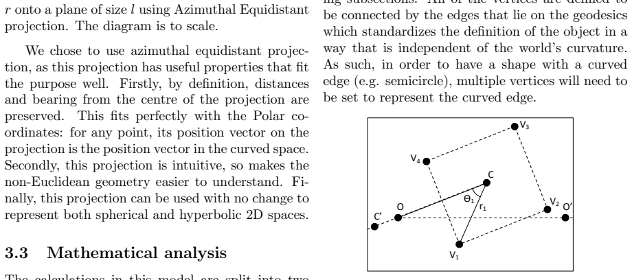
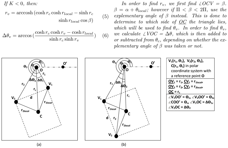
The load-bearing identities are the spherical law of cosines, $\cos(c/r) = \cos(a/r)\cos(b/r) + \sin(a/r)\sin(b/r)\cos C$, and its hyperbolic counterpart $\cosh(c/k) = \cosh(a/k)\cosh(b/k) - \sinh(a/k)\sinh(b/k)\cos C$, with radius $r=1/\sqrt{K}$ or $k=1/\sqrt{-K}$. They are applied to the triangle formed by the global origin, the object centre, and each vertex, which yields the vertex's global polar coordinates; the same rules insert intermediate points along a geodesic edge and advance a moving object along its trajectory. The azimuthal equidistant projection then maps each global polar vector straight onto the screen, preserving distance and bearing from the screen centre, which is why one rendering pipeline works unchanged for both spherical and hyperbolic space.

What would settle it

Take a fixed configuration (known $K$, object position, and local vertex parameters), compute a vertex's global polar coordinates by hand from equations (3)-(6), and compare them with the screen coordinates the engine produces; any mismatch beyond floating-point rounding would refute the rendering claim, and any visible jump at the disc boundary other than the stated antipodal teleport would refute the continuity claim.

Watch

Extended reading notes

Core claim

The central claim is that all geometric calculations can be reduced to the spherical and hyperbolic laws of cosines applied to a triangle whose corners are the global origin, the object centre, and one vertex of the shape. Given the object's global polar position $(r_c,\theta_c)$ and a vertex's local polar position $(r_{\text{local}},\theta_{\text{local}})$, equations (3)-(6) give the vertex's global coordinates; the same identities find edge lengths, intermediate points along geodesics, and the new position of an object moving along its geodesic. Because the azimuthal equidistant projection preserves distance and bearing from the centre of the screen, the computed polar coordinates are used directly as screen positions. Thus the paper claims that any constant-curvature world in the range $-1 \le K \le 1$ can be rendered, and that $K$ can be changed on the fly by simply recomputing every point with the current value.

Load-bearing premise

The visible world is only a finite disc: any object whose centre crosses the disc boundary is teleported to the antipodal point, so the renderer never displays the full non-Euclidean space and the teleport is an artificial discontinuity at the edge.

Editorial extensions

If this is right

A single code path renders Euclidean, spherical, and hyperbolic worlds; switching geometry is just changing the scalar $K$.
Curvature can be swept continuously from $K=1$ to $K=-1$ while objects move, so viewers can watch geodesics bend through flat space without pausing the engine.
Shapes are authored once in local polar coordinates and their vertices are recomputed under the current curvature, so the same object definition works in all three geometries.
Per-frame cost is $O(s \cdot v \cdot i)$ for $s$ shapes with $v$ vertices and tessellation level $i$, and motion updates cost $O(n)$ per object, making real-time rendering feasible for moderate scenes.

Reading between the lines

Editorial extensions of the paper, not claims the author makes directly.

A natural extension is to re-centre the polar reference point on the camera each frame, turning the disc into a moving local chart and removing the antipodal teleport for the observed object.
The same triangle-based identities could be used for ray marching: step a ray along the local geodesic instead of tessellating shapes, which would let curved-space rendering scale per pixel rather than per shape vertex.
If the method is extended to non-constant curvature, the single-triangle cosine law must be replaced by integrating the geodesic equation, so the real-time dial works precisely because curvature is a global constant.
The antipodal teleport can be read as identifying opposite points of the disc, effectively turning the rendering space into a projective or elliptic-like quotient; whether that matches the intended geometry is a testable design choice.

Share X Bluesky LinkedIn Reddit HN

Signed reviews

No signed human review yet.

Editorial analysis

A structured set of objections, weighed in public.

Desk editor's note, referee report, and a circularity audit.

Desk Editor's Note

read the letter

First thing you should know: this is a short graphics paper with a genuinely neat idea — render both spherical and hyperbolic 2D spaces in real time using polar coordinates and an azimuthal equidistant projection, with curvature changeable on the fly. The math is standard spherical/hyperbolic trig, but the packaging is a new application and the video evidence looks credible.

What is new: the unified projection makes the curvature knob trivial, and the complexity analysis is honest. I also give them credit for stating the finite-disc cutoff and antipodal teleport explicitly in Section 3.3 and again in Results, even though it undercuts the 'faithful full-space' phrasing in the abstract.

The soft spots are real, and they bite. Equations (12) and (17), the hyperbolic edge length and intermediate radial coordinate, are printed with the wrong sign (or at least a missing minus sign) — the hyperbolic cosine rule requires cosh c = cosh a cosh b − sinh a sinh b cos C, and the printed text is not that. The stress-test example is correct: r1=r2=1, Δθ=π/3 gives d≈1.11 vs ≈1.78 with the printed form. Same for (17). And (22)–(24) are printed as arccos of hyperbolic expressions, which is another typo for arccosh. Also the definition k=1/sqrt(K) for K<0 is just wrong. These are not cosmetic; if the engine actually executes the printed formulas, it would not render hyperbolic geodesics. If it executes the correct formulas, then the paper does not describe its own method. Either way the central reproducibility claim fails. No code or data is given, so I cannot tell which case holds.

Minor issues: no measured frame rates or benchmarks for 'real-time', and the tessellation level and cutoff distance are the only free parameters, so the claim of arbitrary curvature in [−1,1] is plausible but not validated numerically.

Who is this for: a graphics or math-visualization audience; it could be a reasonable workshop paper or educational note. It is not a research breakthrough, but it is not incoherent — the derivations mostly follow the correct pattern and the limitations are acknowledged. If I were the editor I would send it to peer review with a request for major revisions: fix the signs, reconcile the notation, and ideally release the source or a reproducible pseudocode. If the authors do that, I would be happy to see it used in courses. As is, I would not cite it in my own work because I cannot trust the formulas.

Recommendation: send to a serious referee, but only after the sign errors are addressed; desk-rejecting would be too harsh for an idea this clear.

Referee Report

3 major / 5 minor

Summary. The paper presents a real-time rendering and physics engine for two-dimensional spaces of constant positive or negative curvature. Object positions, velocities, and shape vertices are stored in polar coordinates relative to a reference point, and global vertex positions are computed with spherical and hyperbolic laws of cosines. Geodesic edges are tessellated into straight screen segments, and an azimuthal equidistant projection maps each point's distance and bearing from the reference point directly to screen coordinates. The curvature K can be changed dynamically during execution. The paper provides the trigonometric derivation, time-lapse images of the engine's output, a complexity analysis of O(s*v*i), and a demonstration video. The main claim is that the method correctly calculates and renders shapes in a 2D space of constant curvature in real time.

Significance. If the algebraic statements were correct, the paper would offer a simple, parameter-free method for real-time non-Euclidean rendering with a unified treatment of spherical and hyperbolic geometry. The use of azimuthal equidistant projection to make the projection independent of the curvature sign is a useful idea for graphics applications, educational visualization, and potential dynamic-curvature tools. The paper explicitly uses standard classical theorems with no fitted parameters, which is a strength because it makes the derivations independently checkable. The complexity analysis and the demonstration via time-lapse images are also positive features. However, the hyperbolic formulas as printed contain sign and function errors that contradict the paper's own statement of the hyperbolic law of cosines; as written, the method cannot be reproduced from the text and the central claim is therefore not yet supported.

major comments (3)

[§3.3.1, Eqs. (12) and (17)] The hyperbolic edge-length and intermediate-point formulas are printed with the wrong sign. Eq. (2) states cosh(c/k) = cosh(a/k) cosh(b/k) - sinh(a/k) sinh(b/k) cos C, but Eq. (12) is d = arccosh(cosh r1 cosh r2 + sinh r1 sinh r2 cos Δθ) and Eq. (17) is ri = arccosh(cosh r1 cosh di + sinh r1 sinh di cos α). With the plus sign, the computed d and ri are larger than the true geodesic values; for example, with r1 = r2 = 1 and Δθ = π/3, Eq. (12) gives d ≈ 1.78 instead of the correct d ≈ 1.11. Since Eq. (17) places every intermediate vertex on a hyperbolic edge, the tessellation described in the paper is not a geodesic tessellation. These equations must be corrected to use the minus sign, and the authors should state explicitly whether the engine code uses the corrected or the printed form.
[§3.3.2, Eq. (22)] The hyperbolic position-update formula is printed with both the wrong inverse function and the wrong sign. Eq. (22) is rt1 = arccos(cosh rt0 cosh rp + sinh rt0 sinh rp cos α), but applying the hyperbolic law of cosines to triangle O C_t0 C_t1 gives rt1 = arccosh(cosh rt0 cosh rp - sinh rt0 sinh rp cos α). As printed, Eq. (22) does not follow from the stated hyperbolic cosine rule and will not produce motion along a geodesic. This is load-bearing because Corollary 4 is the basis for the reported physics of object movement.
[§3.3, definition of k] The definition k = 1/√K for K < 0 is invalid because √K is not real for negative K; it must be k = 1/√(−K). Without this correction, every hyperbolic formula that scales lengths by k is undefined. This is a typographical issue in a load-bearing definition, since it affects all hyperbolic equations in the paper.

minor comments (5)

[§3.3.1 and §3.3.2, Eqs. (6), (16), (18), (23), (24)] Several printed fractions are missing parentheses and are ambiguous; for example, Eq. (23) should be written Δθ = arccos((cosh rt0 cosh rt1 − cosh rp)/(sinh rt0 sinh rt1)). Please add parentheses to all quotient formulas.
[§3.1] The phrase "the centre of the of the screen" contains a duplicated article; it should read "the centre of the screen."
[§3.3.1] The word "geodsic" appears instead of "geodesic" in the sentence introducing tessellation.
[§4.1 and §3.3] The paper should more explicitly state in the abstract or introduction that the rendered world is a finite disc with a teleport at the boundary, since this is a deviation from the full non-Euclidean plane and is only mentioned later in the method and results sections.
[References [2], [3]] References [2] and [3] are informal web sources with unstable URLs, and the URL in [2] appears malformed; please replace them with stable persistent identifiers or archival links where possible.

Circularity Check

0 steps flagged · score 0.0 of 10

No significant circularity: the derivation is a direct application of external spherical and hyperbolic cosine laws, with no fitted parameters and no load-bearing self-citation.

full rationale

The paper's derivation chain is self-contained in the sense that its inputs are object state (position, velocity, rotation, local vertex coordinates) and its outputs are global vertex coordinates, geodesic edge tessellation points, and updated motion. The global-coordinate formulas (3)-(6) and edge-tessellation formulas (11)-(18) are direct applications of the spherical law of cosines (Eq. 1) and hyperbolic law of cosines (Eq. 2), both quoted from external classical references [7] and [8]. No parameter is fitted to the rendered output, and no target result is inserted into the equations by construction. The use of azimuthal equidistant projection is a representational design choice: because the projection preserves distance and bearing from the center by definition, the screen placement of a point equals its polar-coordinate position vector; this is an engineering convenience, not a circular derivation of the geometry. The only self-citation is the companion video [9], which is illustrative and not load-bearing for any claimed mathematical result. The paper explicitly acknowledges a limitation: the visible world is cut off at an arbitrary circle and objects are teleported to the antipodal point (Section 3.3 and Results). That truncation weakens the claim of rendering the full non-Euclidean space, but it is a stated limitation, not a circular step. The skeptic's concern about possible sign errors in Eqs. (12) and (17) is a correctness/reproducibility issue, not an instance of circularity: even if those printed formulas are wrong, they are not equivalent to their inputs by definition. The derivation does not rely on a self-citation chain or on renaming a known empirical pattern, so the appropriate circularity score is 0.

Assumptions & free parameters 2 free parameters · 4 assumptions · 0 invented entities

The method rests entirely on standard spherical and hyperbolic trigonometry and the defining property of azimuthal equidistant projection. There are no newly invented particles, forces, or mathematical entities, and no free parameters that are fitted to data. The two implementation-specific parameters (tessellation level and world cutoff) are user choices that do not affect the geometric derivation.

free parameters (2)

tessellation level i
Number of subdivisions per edge is chosen by the implementer. It affects rendering detail and computational cost, but is not fitted to data and does not influence the geometric correctness.
world cutoff distance N (pixels)
Arbitrary limit on the visible radius. Objects are teleported to the antipodal point when crossing it, as described in Section 3.3. This is a user-specified rendering parameter, not a fitted physical constant.

assumptions (4)

standard math Spherical law of cosines (Theorem 1)
Used in equations (3), (4), (11), (13)-(15), and (19)-(21) to compute vertex positions, edge lengths, and object movement on a sphere.
standard math Hyperbolic law of cosines (Theorem 2)
Used in equations (5), (6), (12), (16)-(18), and (22)-(24) for the corresponding hyperbolic space computations.
domain assumption Azimuthal equidistant projection preserves distances and bearings from the center
Section 3.2 states that 'distances and bearing from the centre of the projection are preserved', which justifies using polar coordinates (r, theta) directly as screen coordinates.
domain assumption Constant curvature K in [-1,1] with K=0 Euclidean
The engine only supports constant curvature within this range, as declared at the start of Section 3.3.1 and in the Results. This restricts the applicability to spaces of uniform positive, zero, or negative curvature.

how reviews work

0 comments

Cite this review

Pith. "Pith review of Rendering Non-Euclidean Geometry in Real-Time Using Spherical and Hyperbolic Trigonometry." pith.science (2026). https://pith.science/paper/BHCAVRVO

@misc{pith2026190801742,
  author       = {Pith},
  title        = {Pith review of: Rendering Non-Euclidean Geometry in Real-Time Using Spherical and Hyperbolic Trigonometry},
  year         = {2026},
  howpublished = {\url{https://pith.science/paper/BHCAVRVO}},
  note         = {Machine review of arXiv:1908.01742}
}

read the original abstract

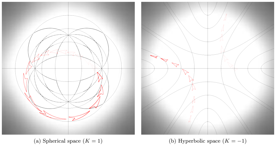
This paper introduces a method of calculating and rendering shapes in a non-Euclidean 2D space. In order to achieve this, we developed a physics and graphics engine that uses hyperbolic trigonometry to calculate and subsequently render the shapes in a 2D space of constant negative or positive curvature in real-time. We have chosen to use polar coordinates to record the parameters of the objects as well as an azimuthal equidistant projection to render the space onto the screen because of the multiple useful properties they have. For example, polar coordinate system works well with trigonometric calculations, due to the distance from the reference point (analogous to origin in Cartesian coordinates) being one of the coordinates by definition. Azimuthal equidistant projection is not a typical projection, used for neither spherical nor hyperbolic space, however one of the main features of our engine relies on it: changing the curvature of the world in real-time without stopping the execution of the application in order to re-calculate the world. This is due to the projection properties that work identically for both spherical and hyperbolic space, as can be seen in the Figure 1 above. We will also be looking at the complexity analysis of this method as well as renderings that the engine produces. Finally we will be discussing the limitations and possible applications of the created engine as well as potential improvements of the described method.

Figures

Figures reproduced from arXiv: 1908.01742 by the authors.

**Figure 2.** Comparison of parallel lines in the 2D spaces of different curvature In spherical geometry all geodesics (straight lines in a non-planar space) intersect, so there are no parallel lines. Even if the lines start parallel, they don’t preserve the same distance along their length and instead appear to ‘bend’ towards each other. In fact any two great circles will intersect twice (unless they are one and the same). Spher… view at source ↗

**Figure 3.** Orthographic projection of the sphere [2] [PITH_FULL_IMAGE:figures/full_fig_p003_3.png] view at source ↗

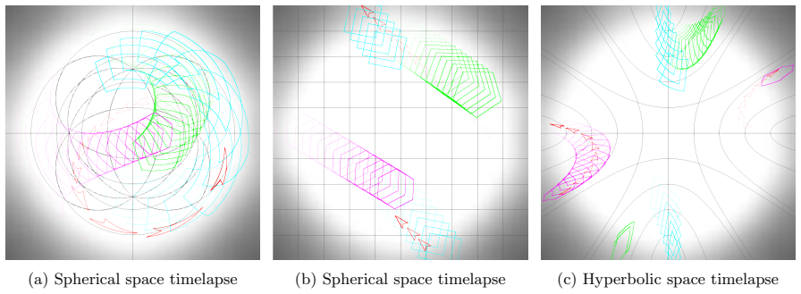
Figures from the paper (12 more)

**Figure 5.** Figure 5: Position of a point A in polar coordinates. [PITH_FULL_IMAGE:figures/full_fig_p004_5.png]

**Figure 6.** Figure 6: Side view of unfolding a sphere or radius [PITH_FULL_IMAGE:figures/full_fig_p005_6.png]

**Figure 7.** Figure 7: Local coordinate system of the object. Key: O, the reference point with coordinates (0, 0); C, position of the object and reference point of the local coordinate system with coordinates (rc, θc); V1, vertex of the illustrated object with local coordinates (r1, θ1); V1…

**Figure 8.** Figure 8: Spherical triangle on the surface of a sphere Theorem 1 For a sphere of radius r and hence Gaussian curvature K = 1 r 2 , as well as a spherical triangle on its surface described by points u, v and w, connected by great circles that form the edges a, b, c (interpreted …

**Figure 10.** Figure 10: Finding the θ and r coordinates of an object’s vertices through a hyperbolic/spherical triangle OCV . Key: O, reference point of the global polar coordinate system with coordinates (0, 0); C, position of the object with coordinates (rc, θc) and origin of the local pol…

**Figure 11.** Figure 11: Finding preliminaries to calculate intermediate points between two vertices: the length of the [PITH_FULL_IMAGE:figures/full_fig_p007_11.png]

**Figure 12.** Figure 12: Finding Intermediate points between two vertices in order to render the edge. Key: O, reference point of the global coordinate system; C, position of the object; V1, V2, vertices of the object; d, edge V1V2; Vi , point on d; r1, r2, ri , r coordinates of the respectiv…

**Figure 13.** Figure 13: Movement of the object along a hyperbolic in Spherical (a) and Hyperbolic (b) space. Orienta [PITH_FULL_IMAGE:figures/full_fig_p008_13.png]

**Figure 14.** Figure 14: Movement along the geodesic orthogonal to the 0 [PITH_FULL_IMAGE:figures/full_fig_p009_14.png]

**Figure 15.** Figure 15: Movement along the geodesic at 45o to the 0o theta vector While these timeline images have the same starting position of the object, these have been used as an aid for visual comparison between images. The software can calculate the object flying in arbitrary directi…

**Figure 16.** Figure 16: Rotation of the object around its centre point [PITH_FULL_IMAGE:figures/full_fig_p010_16.png]

**Figure 17.** Figure 17: Movement of the object while changing the curvature from K=-1 to K=1 In the time-lapse image above ( [PITH_FULL_IMAGE:figures/full_fig_p011_17.png]

Discussion (0). Continue with ORCID to comment.

Reference graph

Works this paper leans on

17 extracted references · 17 canonical work pages

[1]

T. L. Heath, Euclid’s Elements. Dover, 1956. (translated)

work page 1956
[2]

Visualizations of the azimuthal orthographic geometry,

C. A. Furuti, “Visualizations of the azimuthal orthographic geometry,” 2012 (accessed August 02, 2018). http://www.progonos.com/furuti/MapProj/Dither/CartHow/HowOrtho/Img/im orthoRays.pngl

work page 2012
[3]

Equilateral triangles,

Tamfang, “Equilateral triangles,” 2011 (accessed August 03, 2018). https://pointatinﬁnityblog.ﬁles.wordpress.com/2018/02/triangle5.png?w=480&h=480

work page 2011
[4]

Todhunter, Spherical Trigonometry For the use of colleges and schools

I. Todhunter, Spherical Trigonometry For the use of colleges and schools. Project Gutenberg License,

work page
[5]

H. S. Carslaw, The Elements of Non-Euclidean Plane Geometry and Trigonometry . Longmans, Green and co., 1916

work page 1916
[6]

Trigonometry in the hyperbolic plane,

T. Traver, “Trigonometry in the hyperbolic plane,” 2014 (accessed December 2017). Manuscript

work page 2014
[7]

Gellert, S

W. Gellert, S. Gottwald, M. Hellwich, H. Kstner, and H. Kstner, The VNR Concise Encyclopedia of Mathematics, 2nd ed. Van Nostrand Reinhold: New York, 1989. ch. 12

work page 1989
[8]

Gray, Non-euclidean geometryA re-interpretation

J. Gray, Non-euclidean geometryA re-interpretation. Historia Mathematica, 1979. 236258

work page 1979

Show all 17 references

[9]

Rendering non-euclidean space in real-time using spherical and hyperbolic trigonometry,

D. Osudin, C. Child, and Y. Hui-He, “Rendering non-euclidean space in real-time using spherical and hyperbolic trigonometry,” 2019. https://youtu.be/A1ZCFh5qfNg

2019
[10]

Multiple-precision zero-ﬁnding methods and the complexity of elementary function evaluation,

R. P. Brent, “Multiple-precision zero-ﬁnding methods and the complexity of elementary function evaluation,” 2010 (accessed August 26, 2018). http://arxiv.org/abs/1004.3412v2

2010 arXiv
[11]

Fast trigonometry functions using lookup tables,

F. Rochet, “Fast trigonometry functions using lookup tables,” 2004 (accessed August 30, 2018). http://www.ﬂipcode.com/archives/Fast Trigonometry Functions Using Lookup Tables.shtml

2004
[12]

Recent research developments in modern cartography in europe,

G. Gartner and H. Huang, “Recent research developments in modern cartography in europe,” Issue 1: EuroCarto 2015 , 2015

2015
[13]

Modelling noneuclidean movement and landscape connectivity in highly structured ecological networks,

C. Sutherland, “Modelling noneuclidean movement and landscape connectivity in highly structured ecological networks,” British Ecological Society, 2014

2014
[14]

Interpolation of temperature in a mountainous region using nonlinear proﬁles and noneu- clidean distances,

C. Frei, “Interpolation of temperature in a mountainous region using nonlinear proﬁles and noneu- clidean distances,” Royal Meteorological Society, 2013

2013
[15]

The ontology and cosmology of non-euclidean geometry,

K. L. Ross, “The ontology and cosmology of non-euclidean geometry,” Friesian School, 2001

2001
[16]

Geometry and astronomy: Pre-einstein speculations of non-euclidean space,

H. Kragh, “Geometry and astronomy: Pre-einstein speculations of non-euclidean space,” Aarhus University, 2012. 12

2012
[1886]

(republished November 12, 2006)

2006

Pith tools

Reviewed August 14, 2026 · model on record in the stance chip above.

[1] [1]

T. L. Heath, Euclid’s Elements. Dover, 1956. (translated)

work page 1956

[2] [2]

Visualizations of the azimuthal orthographic geometry,

C. A. Furuti, “Visualizations of the azimuthal orthographic geometry,” 2012 (accessed August 02, 2018). http://www.progonos.com/furuti/MapProj/Dither/CartHow/HowOrtho/Img/im orthoRays.pngl

work page 2012

[3] [3]

Equilateral triangles,

Tamfang, “Equilateral triangles,” 2011 (accessed August 03, 2018). https://pointatinﬁnityblog.ﬁles.wordpress.com/2018/02/triangle5.png?w=480&h=480

work page 2011

[4] [4]

Todhunter, Spherical Trigonometry For the use of colleges and schools

I. Todhunter, Spherical Trigonometry For the use of colleges and schools. Project Gutenberg License,

work page

[5] [5]

H. S. Carslaw, The Elements of Non-Euclidean Plane Geometry and Trigonometry . Longmans, Green and co., 1916

work page 1916

[6] [6]

Trigonometry in the hyperbolic plane,

T. Traver, “Trigonometry in the hyperbolic plane,” 2014 (accessed December 2017). Manuscript

work page 2014

[7] [7]

Gellert, S

W. Gellert, S. Gottwald, M. Hellwich, H. Kstner, and H. Kstner, The VNR Concise Encyclopedia of Mathematics, 2nd ed. Van Nostrand Reinhold: New York, 1989. ch. 12

work page 1989

[8] [8]

Gray, Non-euclidean geometryA re-interpretation

J. Gray, Non-euclidean geometryA re-interpretation. Historia Mathematica, 1979. 236258

work page 1979