Acceleration of RANS Solver Convergence via Initialization with Wake Extension Models

Christopher R. Schrock; Eric M. Wolf; Kazuko W. Fuchi; Philip S. Beran

REVIEW 3 major objections 4 minor 31 references

Acceleration of RANS Solver Convergence via Initialization with Wake Extension Models

T0 review · 3 major / 4 minor · reviewed 2026-08-10 · deepseek-v4-flash

Challenge this review Re-run · record.json Download PDF Read on arXiv ↗ Review JSON

Pith's one-line read A CNN wake-extender trained on one flow solution cuts RANS solver wall-clock time 16.4x when used as initialization.

desk verdict A cleanly-demonstrated upper bound: the speedup is real for the stated setup, but the abstract needs the caveat that the initialization is built from the target solution itself. read the letter →

arxiv 2501.14699 v1 pith:BNNPZJ2Q submitted 2025-01-24 physics.flu-dyn cs.NAmath.NAphysics.comp-ph

Kazuko W. Fuchi , Eric M. Wolf , Christopher R. Schrock , Philip S. Beran This is my paper · ORCID

classification physics.flu-dyncs.NAmath.NAphysics.comp-ph

keywords RANSconvergenceaccelerationwakeextensionmodelconvolutionalneuralnetworkCFDinitializationpartitionofunityNACA0012turbulentflowOpenFOAMSpalart-Allmaras

verification ladder T0 review T1 audit T2 compute T3 formal

The pith

A machine-rendered reading of the paper's core claim, the machinery that carries it, and where it could break.

The reading

This paper asks whether a RANS solver for external turbulent flow can be warm-started more effectively by modeling the downstream wake, not just the region near the body. It proposes a convolutional neural network that ingests flow profiles on a slice and predicts how those profiles change a short distance downstream; repeated application extends the wake to the outflow boundary. In a turbulent NACA0012 test case, initializing the solver with the resulting full-domain field took 26.3x fewer iterations and 16.4x less wall-clock time than starting from freestream flow. The paper stresses that these numbers are an upper bound, because the near-body field in the experiment was taken from the exact high-fidelity solution rather than from a learned model.

What carries the argument

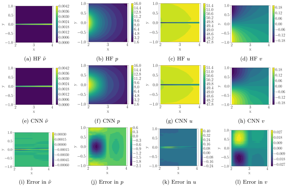
The load-bearing object is the partition-of-unity (POFU) blend $\tilde{q} = W_N \tilde{q}_N + (1-W_N)[W_W \tilde{q}_W + (1-W_W) \tilde{q}_O]$, where smooth window functions select the near-body, wake, and off-body model predictions and sum to one over $\mathbb{R}^2$. The wake model itself is a CNN that takes the field values $q(x_i)$ at $n$ points on a vertical slice and predicts the field increment $\Delta q_i = q(x_{i+1})-q(x_i)$; the field one step downstream is reconstructed as $q(x_{i+1}) = q(x_i)+h(q(x_i))$, and this step is repeated recursively across the wake. Training minimizes the mean squared error between predicted and true increments over $m$ slices from a single high-fidelity solution. The CNN therefore converts a one-slice profile into a full wake to the downstream mesh boundary, and the POFU construction lets that wake be combined smoothly with whatever near-body model is available.

What would settle it

Repeat the NACA0012 test at Re = 6e6, M = 0.15 using the same OpenFOAM simpleFoam/Spalart-Allmaras settings, truncate the near-body field at $x_{\mathrm{interface}}=10$, append the CNN-trained wake to the boundary, and count iterations to the $1\times10^{-7}$ residual target; if the solver does not converge in roughly 1,400 iterations, the reported acceleration does not reproduce.

Watch

Extended reading notes

Core claim

The central claim is that the downstream wake, which prior initialization models often truncate or replace with freestream conditions, is the main obstacle to fast RANS convergence, and that a cheap recursive CNN can remove that obstacle. The authors decompose the domain into near-body, wake, and off-body regions, blend the three predictions with partition-of-unity functions, and use a CNN to map the flow profile at one x-slice to the change in that profile over a downstream step. Training needs only the converged solution of one simulation; the trained model is rolled out recursively from the near-body/wake interface to the downstream boundary. With the high-fidelity solution used as the near-body model, this initialization reaches the $1\times10^{-7}$ residual target in about 1,400 iterations whereas freestream initialization requires 36,887, corresponding to a 16.4x wall-clock speedup. Simpler wake treatments (freestream, uniform extension) only accelerate convergence when the near-body/wake interface is placed far downstream, whereas the CNN model helps even when the interface is close to the body.

Load-bearing premise

The demonstration assumes the near-body flow is already known accurately: the paper uses the interpolated high-fidelity converged solution as the near-body model, so the initialization is already close to the target RANS answer before the wake model is added.

Editorial extensions

If this is right

For the demonstrated NACA0012 turbulent case, full-domain initialization with the CNN wake model reaches convergence in about 1,400 iterations versus 36,887 from freestream, a 26.3x reduction.
Wall-clock time drops 16.4x, making warm-started RANS much cheaper to embed in design loops.
The extent of wake coverage matters more than the wake model choice: simple wake treatments need a far-downstream interface, while the CNN model works from $x_{\mathrm{interface}}=2.0$ onward and peaks at $x_{\mathrm{interface}}=10.0$.
One converged simulation is enough to train the wake model, so data collection cost is one CFD run rather than a large dataset.
The measured accelerations are an upper bound under an exact near-body model, so achievable speedups with learned near-body surrogates will be lower.

Reading between the lines

Editorial extensions of the paper, not claims the author makes directly.

If the near-body surrogate is a learned model with realistic errors, the 16.4x figure likely shrinks; the method's practical value depends on the quality of that surrogate, not just the wake model.
The same slice-to-increment CNN idea could be lifted to three-dimensional wakes by treating each spanwise plane as a slice, although recursive rollout error would need monitoring over long distances.
A testable extension is a parametric study varying angle of attack, Reynolds number, and Mach number to see how far the wake model generalizes beyond its single training condition.
The result points toward initialization research that budgets modeling effort by region, spending the hardest learning on the near-body field and a cheap recurrent model on the wake, rather than learning the full domain at once.

Share X Bluesky LinkedIn Reddit HN

Editorial analysis

A structured set of objections, weighed in public.

Desk editor's note, referee report, and a circularity audit.

Desk Editor's Note

read the letter

Read it. The useful new idea here is the recursive slice-to-slice CNN wake extender: instead of predicting the whole domain or a near-body box, it maps one wake slice to the next and rolls out downstream. Training from a single CFD simulation is a real practical advantage, and the parametric study of the wake-interface location tells you something actionable: the downstream extent of the near-body region is what controls acceleration, and simple freestream or uniform wake extension only work when the near-body region already covers most of the wake. That finding is the paper's best contribution.

The paper is also honest in an important way. It explicitly labels the near-body model as interpolated high-fidelity solution and calls the result an upper bound (Sec. 2 and Sec. 3.2). The convergence histories and wall-clock measurements are shown, the POFU construction is clearly explained, and the numbers are internally consistent.

Now the soft spot, and it is load-bearing for practical interpretation. The near-body field is the converged target solution, and the CNN is trained on downstream changes computed from that same converged solution, then used to reconstruct that same wake. So the 26.3x iteration and 16.4x wall-clock speedups measure how fast the solver converges when you already have a near-exact copy of the answer. The abstract states the speedups without that caveat. The paper labels the near-body assumption an upper bound, but it does not explicitly fold in the wake model's dependence on the target solution. Also, there is one test case, no out-of-sample evaluation, no repeated runs, and no error bars. Those are not fatal for an upper-bound study, but they mean the practical claim is conditional on future tests with a learned near-body model and unseen conditions.

Minor points: the CNN architecture is routine, but that is fine—the contribution is the wake-extension formulation, not the network design. No code or data are provided, which limits reproducibility, but for an AFRL report that is not unusual.

Who is this for? Researchers working on ML-based warm-starting of CFD solvers, and design-loop people who care about RANS initialization costs. It deserves a serious referee: the method is new enough, the single-case demonstration is clean, and the wake-extent sensitivity result is worth publishing. A referee should push for a more careful abstract and one out-of-sample test, but this is not a desk reject.

Referee Report

3 major / 4 minor

Summary. The paper proposes using a convolutional neural network as a wake-extension model to initialize steady RANS simulations of external flow. The computational domain is split into near-body, wake, and off-body regions, and fields from separate models are blended with partition-of-unity functions. The CNN is trained on slices of a single converged high-fidelity simulation and is applied recursively to predict the wake downstream of a user-selected interface. In the numerical demonstration for turbulent flow around a NACA0012 airfoil, the near-body field is taken from the interpolated converged solution, and the CNN wake model is trained on that same solution. The authors report 26.3x fewer iterations and a 16.4x wall-clock speedup relative to freestream initialization, and they conclude that maximal acceleration requires representing the wake to the downstream boundary. The paper explicitly labels the near-body choice as an upper bound on near-body model quality, but the wake model is also trained on and evaluated against the same converged solution used as the initialization target.

Significance. If the claimed acceleration holds under realistic conditions, the proposed decomposition and single-simulation training strategy would be a useful contribution to the CFD initialization literature, where previous CNN-based warm-start methods report roughly 2-4x speedups. The paper is clearly written, provides detailed training and solver settings, and includes convergence histories and comparisons among three wake models. The wake-extension idea is interesting and the three-region POFU formulation is a clean way to combine near-body, wake, and freestream models. However, the headline speedup is currently an in-sample upper bound: both the near-body field and the CNN training data are derived from the converged target solution, so the experiment measures the benefit of starting from a near-exact copy of the target state. The manuscript does not yet demonstrate acceleration in a setting where the target solution is not already available, which is the setting that matters for the stated application.

major comments (3)

[Sec. 2, Sec. 3.1.2, Sec. 3.2] The experimental setup is circular with respect to the central acceleration claim. In Sec. 3.2 the near-body model is the interpolated high-fidelity converged solution, and in Sec. 3.1.2 the CNN wake model is trained on slices of that same converged solution using Eq. (3) with delta-q values computed from the HF solution. The initialization is therefore constructed from the target solution itself, before the wake model is even applied. The paper honestly notes in Sec. 2 and Sec. 3.2 that the near-body choice gives an upper bound, but the same caveat applies to the wake model because its training data come from the target solution. The abstract and conclusion state the 26.3x/16.4x results without this caveat. To support the practical claim, at least one experiment is needed in which neither the near-body field nor the CNN training data come from the converged solution that is being warmed up.
[Sec. 3.2, Figs. 14-16] The speedup estimate is based on a single converged solution and a single baseline run, with no repeated trials or error bars. Because the convergence criterion (residual 1e-7) and wall-clock time can be sensitive to run-to-run variation, solver state, and system load, the quantitative reliability of the reported 16.4x wall-clock speedup is not established. The interface-location sweep provides some related data, but every point still uses the same HF solution and same single baseline. Reporting at least a small number of repeated runs, or bootstrapped statistics over initialization fields, would materially strengthen the claim.
[Sec. 3.2, Sec. 4] The conclusion that maximal acceleration requires representing the entire wake to the downstream boundary is derived entirely from experiments with an interpolated HF near-body field. With a realistic learned near-body model, errors in the near-body field will be propagated and potentially amplified by the recursive CNN rollout in Algorithm 1, so the conclusion may not transfer. The paper should either test the wake model with a perturbed or approximate near-body field or explicitly restrict the conclusion to the perfect-near-body upper-bound setting.

minor comments (4)

[Appendix, Eq. (8)] The transition function T(r) as printed, 6r^5 - 15r^4 + 1 - r^3, is not the standard smoothstep function; it does not satisfy T(1/2)=1/2 and may not be C^1 at the endpoints. Please check the formula, which should likely be 6r^5 - 15r^4 + 10r^3.
[Sec. 2.3] The text refers to a 'NACA0102 airfoil'; this appears to be a typo for NACA0012, as used elsewhere in the paper.
[Sec. 3.2] The sentence 'The residuals for the CFD runs using the CNN model are plotted without the comparison to standard runs in Fig. 14 for a closer look' should refer to Fig. 16(c) and (d), not Fig. 14, which shows iterations versus interface location.
[Sec. 1, reference [29]] Reference [29] is listed as a preprint without a year or repository identifier; please provide the arXiv identifier or update the citation if it has been published.

Circularity Check

2 steps flagged · score 6.0 of 10

The 26.3x/16.4x speedup is an in-sample upper bound: the wake model is trained on the converged target solution's own slice-to-slice differences and then used to reconstruct that same solution as the initialization.

fitted input called prediction [Sec. 2.2.3 (Eq. (3), Algorithm 1) and Sec. 3.1.2]
"The loss function for the model training is defined as: L = 1/m Σ ||∆qi − h(q(xi))||2 ... The CNN training data is generated using ∆ q0, ∆q1, · · ·, ∆qm−1 from the HF solution."

The CNN h is trained on the target HF solution's own slice-to-slice changes Δq_i. Algorithm 1 then initializes the wake by recursively applying h starting from q(x0), which in the experiment is evaluated from the same HF solution. Thus the 'predicted' downstream wake is a reconstruction of the training target, not a prediction of an unknown flow. The measured 26.3x/16.4x acceleration therefore measures the cost of starting from a near-exact copy of the converged solution, so the central speedup claim is an in-sample fit rather than an independent demonstration.
fitted input called prediction [Sec. 2 (near-body surrogate) and Sec. 3.2]
"in order to establish an upper bound on performance in the CFD initialization task with respect to near-body model quality, interpolated high-fidelity (HF) solution data is used as a surrogate near-body model in the numerical experiments presented in this work. ... To isolate the impact of the wake model and the POFU window selection from the effects of the near-body model accuracy, interpolated HF solution is used as the near-body model in the following studies."

The near-body model in the actual demonstration is the converged target solution itself, interpolated onto the mesh; the wake model is trained on the same solution. Consequently, the initialization field is built from the exact answer the RANS solver is supposed to find. The paper openly labels this an upper bound for the near-body component, but the abstract states the 16.4x speedup without this qualification, and the wake model's dependence on the target solution is not included in the stated caveat. The comparison is thus between warm-starting from the target solution and cold-starting from freestream, which is forced by construction.

full rationale

No load-bearing self-citation chains or imported uniqueness theorems are present; the central difficulty is experimental in-sample reconstruction. The paper is methodologically honest in Secs. 2 and 3.2 that the near-body model is interpolated high-fidelity solution data, but the CNN wake extender is trained on and evaluated against the same high-fidelity solution, and the recursive application in Algorithm 1 reconstructs that same wake. Thus the reported acceleration is an upper bound for a warm start that already knows the converged answer, and it does not demonstrate acceleration for a RANS solve whose target is unknown. Because this is disclosed as an upper bound rather than concealed, the circularity is partial rather than complete; the score reflects that the headline speedup reduces by construction to an in-sample fit.

Assumptions & free parameters 4 free parameters · 4 assumptions · 0 invented entities

The central claim is a numerical demonstration, so the ledger is dominated by modeling choices rather than physical postulates. The key uncounted inputs are the hyperparameters and domain decomposition choices, plus the assumption that the target converged solution can be used to build the warm start.

free parameters (4)

CNN hyperparameters (kernel size 2, 3 conv blocks, batch size 8, initial learning rate 1e-3, cosine annealing T0=10…
Chosen by hand rather than derived; the model behavior and training cost depend on them, and no systematic tuning study is reported.
Training grid parameters: n=128 y-points, slice spacing Δx=1.0, y-range [-1,1], start slice x0=2.0 = n=128, Δx=1.0, y in [-1,1], x0=2.0
These choices set the resolution and downstream extent of the CNN wake model and are not varied or justified except as defaults.
POFU transition widths sx, sy
The window functions in the Appendix depend on sx and sy, but the values used in the CFD initialization study are not reported, so the blending behavior is underspecified.
Near-body/wake interface location x_interface = 2.0 to 100.0
The method requires choosing where the near-body model ends and the wake model begins; the reported acceleration depends strongly on this location (Fig. 14).

assumptions (4)

domain assumption 2D incompressible RANS with the Spalart-Allmaras turbulence model adequately represents the NASA NACA0012 validation case at Re=6e6 and M=0.15.
Used to generate the high-fidelity solution that is both the training data and the initialization target; Section 3.1.1.
domain assumption The OpenFOAM simpleFoam converged solution with the settings in Table 1 is an accurate enough reference for the CFD initialization task.
The interpolated converged solution serves as both the near-body surrogate and the CNN training target; any error in this reference propagates into the evaluation.
ad hoc to paper The wake evolution is Markovian in x: q(x_i + Δx) depends only on q(x_i) via the learned h.
Equation (2) and Algorithm 1 recursively march the wake slice by slice; this assumption is necessary for the CNN method and is not independently validated.
ad hoc to paper A single converged simulation provides enough diversity to train a wake model that is useful for the same flow condition.
The model is trained and evaluated on the same case; no out-of-sample experiment is performed, so this assumption is untested.

how reviews work

0 comments

Cite this review

Pith. "Pith review of Acceleration of RANS Solver Convergence via Initialization with Wake Extension Models." pith.science (2026). https://pith.science/paper/BNNPZJ2Q

@misc{pith2026250114699,
  author       = {Pith},
  title        = {Pith review of: Acceleration of RANS Solver Convergence via Initialization with Wake Extension Models},
  year         = {2026},
  howpublished = {\url{https://pith.science/paper/BNNPZJ2Q}},
  note         = {Machine review of arXiv:2501.14699}
}

read the original abstract

Use of appropriate initialization to warm-start Reynolds-averaged Navier-Stokes (RANS) simulations of turbulent flow can facilitate convergence and lead to efficient use of computational resources. In this work, a method to model downstream wake development in external turbulent flow is proposed and used for RANS solver convergence acceleration. To balance the model accuracy and cost, the proposed method divides the analysis domain into three regions: near-body, wake and off-body. An approach based on a convolutional neural network is introduced as an efficient method to predict the downstream wake development. The model training only requires data from a single simulation, and its use is demonstrated to be effective in accelerating the RANS simulation when combined with an accurate flow prediction in the near-body region. The simulation using the proposed method took 26.3x fewer iterations, achieving 16.4x speedup in wall-clock time, compared to a baseline run using freestream initialization.

Figures

Figures reproduced from arXiv: 2501.14699 by the authors.

**Figure 3.** Examples of flow field using different wake models: (a) freestream conditions, (b) uniform wake [PITH_FULL_IMAGE:figures/full_fig_p004_3.png] view at source ↗

**Figure 4.** CNN model is used to predict the field difference downstream. [PITH_FULL_IMAGE:figures/full_fig_p005_4.png] view at source ↗

Figures from the paper (12 more)

**Figure 5.** Figure 5: Wake extension through the recursive use of CNN model. [PITH_FULL_IMAGE:figures/full_fig_p005_5.png]

**Figure 6.** Figure 6: CNN architecture used for the wake extension model. [PITH_FULL_IMAGE:figures/full_fig_p006_6.png]

**Figure 7.** Figure 7: CNN wake model output is interpolated onto CFD mesh. [PITH_FULL_IMAGE:figures/full_fig_p006_7.png]

**Figure 8.** Figure 8: Flow of operations for model-based CFD initialization. [PITH_FULL_IMAGE:figures/full_fig_p007_8.png]

**Figure 9.** Figure 9: HF solution for incompressible turbulent flow around NACA0012 airfoil at [PITH_FULL_IMAGE:figures/full_fig_p009_9.png]

**Figure 10.** Figure 10: Loss function evolution for the wake extension model training. [PITH_FULL_IMAGE:figures/full_fig_p010_10.png]

**Figure 11.** Figure 11: Flow field y−profiles of the wake, compared between prediction by the CNN model (solid) and data (dots). gion, the interface location has a severe impact on the acceleration achieved. The leftmost data in [PITH_FULL_IMAGE:figures/full_fig_p011_11.png]

**Figure 12.** Figure 12: Comparison between HF and CNN-predicted wake at [PITH_FULL_IMAGE:figures/full_fig_p012_12.png]

**Figure 13.** Figure 13: Comparison between HF and CNN-predicted wake at [PITH_FULL_IMAGE:figures/full_fig_p013_13.png]

**Figure 14.** Figure 14: Comparison of CFD steps to convergence using different wake models in initialization. [PITH_FULL_IMAGE:figures/full_fig_p013_14.png]

**Figure 15.** Figure 15: Comparison of CFD wall-clock time to convergence using different wake models in initialization. [PITH_FULL_IMAGE:figures/full_fig_p014_15.png]

**Figure 16.** Figure 16: Convergence history for CFD runs using freestream vs CNN wake model initialization. [PITH_FULL_IMAGE:figures/full_fig_p014_16.png]

Discussion (0). Continue with ORCID to comment.

Reference graph

Works this paper leans on

31 extracted references · 20 canonical work pages

[1]

Computational fluid dynamics: the basics with applications

D Anderson John Jr. “Computational fluid dynamics: the basics with applications”. In: Science/Engineering/Math. McGraw-Hill Science (1995)

work page 1995
[2]

Best practices for reduction of uncertainty in CFD results

Michael Mendenhall, Robert Childs, and Joseph Morrison. “Best practices for reduction of uncertainty in CFD results”. In: 41st Aerospace Sciences Meeting and Exhibit . 2003, p. 411. 13 Figure 15: Comparison of CFD wall-clock time to convergence using different wake models in initialization. (a) Freestream vs CNN model rollout A (b) Freestream vs CNN model...

work page 2003
[3]

Verification and Validation in Scientific Computing

William L Oberkampf and Christopher J Roy. Verification and Validation in Scientific Computing . 2010

work page 2010
[4]

Convolutional Neural Networks for Steady Flow Approxi- mation

Xiaoxiao Guo, Wei Li, and Francesco Iorio. “Convolutional Neural Networks for Steady Flow Approxi- mation”. In: Proceedings of the 22nd ACM SIGKDD International Conference on Knowledge Discovery and Data Mining. KDD ’16. San Francisco, California, USA: Association for Computing Machinery, 2016, 14 pp. 481–490. isbn: 9781450342322. doi: 10.1145/2939672.293...

arXiv 2016
[5]

On the role and challenges of CFD in the aerospace industry

P. R. Spalart and V. Venkatakrishnan. “On the role and challenges of CFD in the aerospace industry”. en. In: The Aeronautical Journal 120.1223 (Jan. 2016), pp. 209–232. issn: 0001-9240, 2059-6464. doi: 10.1017/aer.2015.10

work page doi:10.1017/aer.2015.10 2016
[6]

SGDR: Stochastic Gradient Descent with Warm Restarts

Ilya Loshchilov and Frank Hutter. SGDR: Stochastic Gradient Descent with Warm Restarts . Tech. rep. arXiv:1608.03983 [cs, math] type: article. arXiv, May 2017. doi: 10.48550/arXiv.1608.03983 . url: http://arxiv.org/abs/1608.03983

arXiv doi:10.48550/arxiv.1608.03983 2017
[7]

State-of-the-art in aerodynamic shape optimisation methods

S. N. Skinner and H. Zare-Behtash. “State-of-the-art in aerodynamic shape optimisation methods”. In: Applied Soft Computing 62 (Jan. 2018), pp. 933–962. issn: 1568-4946. doi: 10.1016/j.asoc.2017.09. 030

work page doi:10.1016/j.asoc.2017.09 2018
[8]

Prediction of Aerodynamic Flow Fields Using Convolutional Neural Networks

Yaser Afshar et al. “Prediction of Aerodynamic Flow Fields Using Convolutional Neural Networks”. en. In: Computational Mechanics 64.2 (May 2019), pp. 525–545. issn: 1432-0924. doi: 10.1007/s00466- 019-01740-0 . arXiv: 1905.13166 [physics.flu-dyn]. url: https://doi.org/10.1007/s00466-019- 01740-0

work page Pith review arXiv 2019

Show all 31 references

[9]

NN-SVG: Publication-Ready Neural Network Architecture Schematics

Alexander LeNail. “NN-SVG: Publication-Ready Neural Network Architecture Schematics”. en. In: Jour- nal of Open Source Software 4.33 (Jan. 2019), p. 747. issn: 2475-9066. doi: 10.21105/joss.00747. url: https://joss.theoj.org/papers/10.21105/joss.00747

2019 doi
[10]

Combining Differentiable PDE Solvers and Graph Neural Networks for Fluid Flow Prediction

Filipe De Avila Belbute-Peres, Thomas Economon, and Zico Kolter. “Combining Differentiable PDE Solvers and Graph Neural Networks for Fluid Flow Prediction”. en. In: (Nov. 2020), pp. 2402–2411. issn: 2640-3498

2020
[11]

CFDNet: A Deep Learning-Based Accelerator for Fluid Simulations

Octavi Obiols-Sales et al. “CFDNet: A Deep Learning-Based Accelerator for Fluid Simulations”. In: Proceedings of the 34th ACM International Conference on Supercomputing . ICS ’20. Barcelona, Spain: Association for Computing Machinery, 2020. isbn: 9781450379830. doi: 10 . 1145 ...

2020
[12]

Generalizability of Convolutional Encoder–Decoder Networks for Aerodynamic Flow-Field Prediction Across Geometric and Physical- Fluidic Variations

Kaustubh Tangsali, Vinayak R. Krishnamurthy, and Zohaib Hasnain. “Generalizability of Convolutional Encoder–Decoder Networks for Aerodynamic Flow-Field Prediction Across Geometric and Physical- Fluidic Variations”. In: Journal of Mechanical Design 143.051704 (Nov. 2020). issn:...

2020 doi
[13]

Deep Learning Methods for Reynolds-Averaged Navier-Stokes Simulations of Airfoil Flows

Nils Thuerey et al. “Deep Learning Methods for Reynolds-Averaged Navier-Stokes Simulations of Airfoil Flows”. In: AIAA Journal 58.1 (2020), pp. 25–36. issn: 0001-1452. doi: 10 . 2514 / 1 . J058291. url: https://doi.org/10.2514/1.J058291

2020 doi
[14]

Physics-informed neural networks (PINNs) for fluid mechanics: a review

Shengze Cai et al. “Physics-informed neural networks (PINNs) for fluid mechanics: a review”. en. In: Acta Mechanica Sinica 37.12 (Dec. 2021), pp. 1727–1738. issn: 1614-3116. doi: 10.1007/s10409-021- 01148-1. url: https://doi.org/10.1007/s10409-021-01148-1

2021 doi
[15]

NSFnets (Navier-Stokes flow nets): Physics-informed neural networks for the incom- pressible Navier-Stokes equations

Xiaowei Jin et al. “NSFnets (Navier-Stokes flow nets): Physics-informed neural networks for the incom- pressible Navier-Stokes equations”. en. In: Journal of Computational Physics 426 (Feb. 2021), p. 109951. issn: 0021-9991. doi: 10.1016/j.jcp.2020.109951. url: https://www.sci...

2021
[16]

A point-cloud deep learning framework for prediction of fluid flow fields on irregular geometries

Ali Kashefi, Davis Rempe, and Leonidas J. Guibas. “A point-cloud deep learning framework for prediction of fluid flow fields on irregular geometries”. In: Physics of Fluids 33.2 (Feb. 2021), p. 027104. issn: 1070-

2021
[17]

SURFNet: Super-Resolution of Turbulent Flows with Transfer Learning us- ing Small Datasets

Octavi Obiols-Sales et al. “SURFNet: Super-Resolution of Turbulent Flows with Transfer Learning us- ing Small Datasets”. In: 2021 30th International Conference on Parallel Architectures and Compilation Techniques (PACT). Sept. 2021, pp. 331–344. doi: 10.1109/PACT52795.2021.00031

2021
[18]

Experience report of physics-informed neural networks in fluid simulations: pitfalls and frustration

Pi-Yueh Chuang and Lorena A. Barba. “Experience report of physics-informed neural networks in fluid simulations: pitfalls and frustration”. In: Proceedings of the 21st Python in Science Conference . Ed. by Meghann Agarwal et al. 2022, pp. 28–36. doi: 10.25080/majora-212e5952-005

2022 doi
[19]

Physics-informed neural networks for solving Reynolds-averaged Navier-Stokes equations

Hamidreza Eivazi et al. “Physics-informed neural networks for solving Reynolds-averaged Navier-Stokes equations”. In: Physics of Fluids 34.7 (July 2022), p. 075117. issn: 1070-6631. doi: 10.1063/5.0095270. url: https://aip.scitation.org/doi/full/10.1063/5.0095270. 15

2022 doi
[20]

Multi-Fidelity Machine Learning Applied to Steady Fluid Flows

Kazuko W. Fuchi et al. “Multi-Fidelity Machine Learning Applied to Steady Fluid Flows”. In: Interna- tional Journal of Computational Fluid Dynamics 36.7 (Aug. 2022), pp. 618–640. issn: 1061-8562. doi: 10.1080/10618562.2022.2154758. url: https://doi.org/10.1080/10618562.2022.2154758

2022
[21]

OpenFOAM v10. en-GB. 2022. url: https://openfoam.org/

2022
[22]

Towards high-accuracy deep learning inference of compressible flows over aerofoils

Li-Wei Chen and Nils Thuerey. “Towards high-accuracy deep learning inference of compressible flows over aerofoils”. en. In: Computers & Fluids 250 (Jan. 2023), p. 105707. issn: 0045-7930. doi: 10 . 1016/j.compfluid.2022.105707 . url: https://www.sciencedirect.com/science/artic...

2023
[23]

Grossmann et al

Tamara G. Grossmann et al. Can Physics-Informed Neural Networks beat the Finite Element Method? Tech. rep. arXiv:2302.04107 [cs, math] type: article. arXiv, Feb. 2023.doi: 10.48550/arXiv.2302.04107. url: http://arxiv.org/abs/2302.04107

2023 doi arXiv
[24]

Fourth AIAA High-Lift Prediction Workshop: Fixed-Grid Reynolds-Averaged Navier–Stokes Summary

Carl F. Ollivier-Gooch and James G. Coder. “Fourth AIAA High-Lift Prediction Workshop: Fixed-Grid Reynolds-Averaged Navier–Stokes Summary”. In: Journal of Aircraft 0.0 (2023), pp. 1–13. issn: 0021-

2023
[25]

Evolutionary Multi-Objective Aerodynamic Design Optimization Using CFD Simulation Incorporating Deep Neural Network

Yukito Tsunoda and Akira Oyama. Evolutionary Multi-Objective Aerodynamic Design Optimization Using CFD Simulation Incorporating Deep Neural Network . Tech. rep. arXiv:2304.14973 [physics] type: article. arXiv, Apr. 2023. doi: 10.48550/arXiv.2304.14973. url: http://arxiv.org/ab...

2023 doi arXiv
[26]

Fast simulation of airfoil flow field via deep neural network

Kuijun Zuo et al. Fast simulation of airfoil flow field via deep neural network . Tech. rep. arXiv:2312.04289 [physics] type: article. arXiv, Dec. 2023. doi: 10.48550/arXiv.2312.04289

2023 doi arXiv
[27]

2D NACA 0012 Airfoil Validation Case

NASA Langley Research Center Turbulence Modeling Resource. 2D NACA 0012 Airfoil Validation Case . url: %7Bhttps://turbmodels.larc.nasa.gov/naca0012%7B%5C_%7Dval.html%7D
[28]

Accuracy Improvement Technique of DNN for Accelerating CFD Simulator

Yukito Tsunoda et al. “Accuracy Improvement Technique of DNN for Accelerating CFD Simulator”. In: AIAA SCITECH 2022 Forum . American Institute of Aeronautics and Astronautics. doi: 10.2514/6. 2022-1437. url: https://arc.aiaa.org/doi/abs/10.2514/6.2022-1437

2022 doi
[29]

Neural operator-based super-fidelity: A warm-start approach for accelerating steady- state simulations

Xu-Hui Zhou et al. “Neural operator-based super-fidelity: A warm-start approach for accelerating steady- state simulations”. (pre-print). Appendix Window Functions in POFU 2D and 1D window functions W2D and W1D in Fig. 2 are defined as W2D (x, y) = T ((x − xmin) /sx) T ((xmax ...
[6631]

url: https://aip.scitation.org/doi/abs/10.1063/5.0033376

doi: 10.1063/5.0033376. url: https://aip.scitation.org/doi/abs/10.1063/5.0033376

doi
[8669]

url: https://doi.org/10.2514/1.C037184

doi: 10.2514/1.C037184. url: https://doi.org/10.2514/1.C037184

doi

Pith tools

Reviewed August 10, 2026 · model on record in the stance chip above.

[1] [1]

Computational fluid dynamics: the basics with applications

D Anderson John Jr. “Computational fluid dynamics: the basics with applications”. In: Science/Engineering/Math. McGraw-Hill Science (1995)

work page 1995

[2] [2]

Best practices for reduction of uncertainty in CFD results

Michael Mendenhall, Robert Childs, and Joseph Morrison. “Best practices for reduction of uncertainty in CFD results”. In: 41st Aerospace Sciences Meeting and Exhibit . 2003, p. 411. 13 Figure 15: Comparison of CFD wall-clock time to convergence using different wake models in initialization. (a) Freestream vs CNN model rollout A (b) Freestream vs CNN model...

work page 2003

[3] [3]

Verification and Validation in Scientific Computing

William L Oberkampf and Christopher J Roy. Verification and Validation in Scientific Computing . 2010

work page 2010

[4] [4]

Convolutional Neural Networks for Steady Flow Approxi- mation

Xiaoxiao Guo, Wei Li, and Francesco Iorio. “Convolutional Neural Networks for Steady Flow Approxi- mation”. In: Proceedings of the 22nd ACM SIGKDD International Conference on Knowledge Discovery and Data Mining. KDD ’16. San Francisco, California, USA: Association for Computing Machinery, 2016, 14 pp. 481–490. isbn: 9781450342322. doi: 10.1145/2939672.293...

arXiv 2016

[5] [5]

On the role and challenges of CFD in the aerospace industry

P. R. Spalart and V. Venkatakrishnan. “On the role and challenges of CFD in the aerospace industry”. en. In: The Aeronautical Journal 120.1223 (Jan. 2016), pp. 209–232. issn: 0001-9240, 2059-6464. doi: 10.1017/aer.2015.10

work page doi:10.1017/aer.2015.10 2016

[6] [6]

SGDR: Stochastic Gradient Descent with Warm Restarts

Ilya Loshchilov and Frank Hutter. SGDR: Stochastic Gradient Descent with Warm Restarts . Tech. rep. arXiv:1608.03983 [cs, math] type: article. arXiv, May 2017. doi: 10.48550/arXiv.1608.03983 . url: http://arxiv.org/abs/1608.03983

arXiv doi:10.48550/arxiv.1608.03983 2017

[7] [7]

State-of-the-art in aerodynamic shape optimisation methods

S. N. Skinner and H. Zare-Behtash. “State-of-the-art in aerodynamic shape optimisation methods”. In: Applied Soft Computing 62 (Jan. 2018), pp. 933–962. issn: 1568-4946. doi: 10.1016/j.asoc.2017.09. 030

work page doi:10.1016/j.asoc.2017.09 2018

[8] [8]

Prediction of Aerodynamic Flow Fields Using Convolutional Neural Networks

Yaser Afshar et al. “Prediction of Aerodynamic Flow Fields Using Convolutional Neural Networks”. en. In: Computational Mechanics 64.2 (May 2019), pp. 525–545. issn: 1432-0924. doi: 10.1007/s00466- 019-01740-0 . arXiv: 1905.13166 [physics.flu-dyn]. url: https://doi.org/10.1007/s00466-019- 01740-0

work page Pith review arXiv 2019