Low-frequency output fluctuations in an open exclusion process with particle pausing

Quentin Thommen

REVIEW 3 major objections 6 minor 36 references

Low-frequency output fluctuations in an open exclusion process with particle pausing

T0 review · 3 major / 6 minor · reviewed 2026-08-12 · deepseek-v4-flash

Challenge this review Re-run · record.json Download PDF Read on arXiv ↗ Review JSON

Pith's one-line read In the open pausing TASEP at reference rates, the long-window Fano factor of exit counts peaks at a mean paused population $N_p\simeq1.5$–$2$ for lattice lengths $L=50$–$500$, with the peak pausing rate scaling as $1/L$.

desk verdict A real and useful discovery—nonmonotonic output noise in the pausing TASEP—honest about its approximations, but the peak location and scaling are reported without uncertainties. read the letter →

arxiv 2608.08074 v1 pith:BQY56XK5 submitted 2026-08-08 cond-mat.stat-mech q-bio.SC

Quentin Thommen This is my paper · ORCID

classification cond-mat.stat-mechq-bio.SC MSC 82C2282C3160K35

keywords TASEPpausingFanofactorlow-frequencynoisefinite-sizescalingtrafficjamsexit-countstatisticsstochastictransport

verification ladder T0 review T1 audit T2 compute T3 formal

The pith

A machine-rendered reading of the paper's core claim, the machinery that carries it, and where it could break.

The reading

This paper asks whether the finite-size pausing regime of an open totally asymmetric exclusion process, previously identified through the mean current, has a distinct signature in the timing of particles leaving the lattice. It establishes that the long-window Fano factor of exit counts is strongly nonmonotonic in the pausing rate: at the reference boundary rates the peak stays at a measured mean paused population $N_p=L\rho_{\rm paused}\simeq1.5$–$2$ for all lattice lengths tested, $L=50$–$500$, while the pausing rate at the peak scales as $k_p^{\max}\propto L^{-1}$. The absolute fluctuation rate $JF_\infty$ is also nonmonotonic, so the relative-noise maximum is not merely a normalization artifact of a decreasing mean current. A minimal constant-birth, linear-death approximation with a two-valued current predicts the maximum at $N_p^\star\simeq1.50$, and the simulations delimit that approximation by showing the pause number is overdispersed and that slower unpausing at fixed $N_p$ raises both the correlation time and the noise amplitude.

What carries the argument

The load-bearing analytical object is a constant-birth, linear-death approximation for the instantaneous number of paused particles $M(t)$, paired with a two-valued output current. Pauses are assumed to appear at a constant rate $\lambda=k_pN_A$ and each paused particle resumes at rate $k_u$, so the stationary count is Poisson with mean $n=\lambda/k_u=N_p$; the current is $J_0$ when no pause is present and $J_p$ otherwise, with $J_p\ll J_0$ in the strong-blocking limit. The covariance of the pause-free indicator gives $F_{\rm slow}(n)\propto e^{-n}[\mathrm{Ei}(n)-\gamma-\ln n]$, where $\mathrm{Ei}$ is the exponential integral, and its maximizing $n$ solves $(e^n-1)/n=\mathrm{Ei}(n)-\gamma-\ln n$, yielding $n^\star\simeq1.50$. Stationary pause balance $k_pN_A=k_uN_p$ then maps this order-one crossover to $k_p^{\max}\propto 1/(\rho L)$, giving the observed $1/L$ scaling of the pausing rate at fixed boundary conditions.

What would settle it

Run the same scan with boundary rates chosen so that the pause-free stationary density is near 0.5 instead of the reference 0.27–0.30; if the Fano-factor maximum then occurs at $N_p$ well above 2, the order-one location is not a generic feature of the finite-size crossover but only of the reference boundary conditions.

Watch

Extended reading notes

Core claim

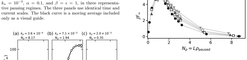
At reference rates $\alpha=0.1$, $\beta=1$, $\epsilon=1$, and $k_u=10^{-3}$, increasing the per-particle pausing rate $k_p$ lowers the stationary current smoothly, but the fitted low-frequency Fano plateau $F_\infty$ rises sharply, peaks near $N_p\simeq1.9$, and then falls. The same order-one paused population locates the maximum for $L=50$, $100$, $200$, $300$, and $500$ even though $k_p^{\max}$ changes by more than a decade, and $Lk_p^{\max}$ stays approximately constant, consistent with $k_p^{\max}\propto L^{-1}$. The product $JF_\infty$, the long-window variance growth rate, is also nonmonotonic and peaks at $N_p$ of order unity, showing the intermittent regime modulates absolute output fluctuations, not just their normalized ratio. The paper stresses that the numerical location is not universal: an $\alpha=0.03$ control preserves the regime but shifts the peak to $N_p\simeq3.26$.

Load-bearing premise

The predicted peak at about 1.5 paused particles assumes pauses appear independently at a constant average rate and that every configuration containing a pause has the same output current; the simulations show pause counts are more variable than that and that the noise amplitude depends on how long pauses last.

Editorial extensions

If this is right

The mean current alone cannot identify the most intermittent regime: the same smooth decrease in $J$ accompanies both weak and maximal relative noise, so exit-count Fano statistics are the discriminating observable.
System size mainly changes the microscopic rate needed to reach the crossover, not the collective variable that locates it; a longer lattice requires a proportionally smaller per-particle pausing rate.
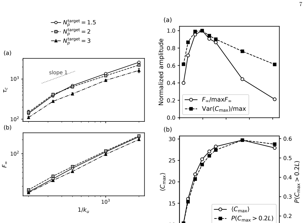
Pause abundance $N_p$ sets the position of the peak at fixed boundary conditions, but not its amplitude; slower unpausing increases both $\tau_c$ and $F_\infty$ at essentially unchanged $N_p$.
Pause-number dynamics supplies the effective clock for output decorrelation, while fluctuations of the largest contiguous cluster are the closest structural correlate of the noise amplitude, suggesting a two-layer mechanism.
For biological transcripts, a fixed mean completion rate can correspond to regular delivery or to productive episodes separated by silent intervals, so downstream processes sensitive to completion times receive different temporal inputs from the same average elongation rate.

Reading between the lines

Editorial extensions of the paper, not claims the author makes directly.

In my reading, the overdispersed pause-number statistics point to a natural refinement: replacing the Poisson immigration-death process with a bursty or exclusion-corrected birth process would shift the predicted optimum away from 1.50, and the model's stored trajectories could be used to test which birth process reproduces the measured peak.
The $\alpha=0.03$ shift suggests that a systematic map of the open-system phase diagram would reveal $N_p^\star$ as a function of boundary-driven density; the paper does not provide such a map.
A testable downstream consequence is that in stochastic gene-expression models, the Fano factor of completed mRNA numbers should inherit the same nonmonotonic dependence on pausing kinetics even when the mean mRNA level is monotonic; this follows from the exit-counting mechanism but is not demonstrated here.

Share X Bluesky LinkedIn Reddit HN

Editorial analysis

A structured set of objections, weighed in public.

Desk editor's note, referee report, and a circularity audit.

Desk Editor's Note

read the letter

This paper is worth reading because it fills a real gap: prior work on the pausing TASEP focused on the stationary current, but nobody had looked at the temporal statistics of the exit process. The main finding is a robust nonmonotonic peak in the low-frequency Fano factor F∞ as a function of the pausing rate. The peak sits at a mean paused population Np ≈ 1.5–2 for L = 50–500, and the pausing rate at the peak scales as L^-1. The absolute fluctuation rate J F∞ is also nonmonotonic, which rules out the boring explanation that the peak is just normalization by a falling current. That is a clean, useful result.

The paper also does something nice analytically: it derives n* ≈ 1.50 for the peak location from an immigration–death approximation, and this is not fitted to the simulations. The authors are upfront that it's a minimal theory, and they show where it fails—the pause number is overdispersed, and the peak position shifts at α = 0.03. The structural analysis (pause-number vs. cluster-size variance) separates the clock from the amplitude and is a good complement to the main claim.

The soft spots are real but not fatal. Table I reports the peak locations to two decimals and F∞ to three significant figures with no error bars. The peak is just the largest plateau on a discrete kp grid, with no interpolation and no test of whether neighboring points are statistically distinguishable. The appendix mentions replicate dispersion, but it's not propagated to these headline numbers. The L^-1 scaling is consistent with the data, but without uncertainties you can't tell whether the slight drift in Np^max (1.94 to 1.86) is meaningful. That's a verification gap, not evidence of error—the effect sizes are large and the robustness checks (window-removal, α=0.03 control) support the qualitative picture. A separate issue: the reproducibility package is announced but not actually accessible.

The Poisson approximation is load-bearing for the explanatory part, but the paper discloses its limits clearly. It doesn't undermine the empirical findings.

Overall: a solid, honest contribution. I'd be happy to referee it. It needs error bars on the key quantitative claims and the data actually made available, but the core result is likely correct.

Referee Report

3 major / 6 minor

Summary. The paper studies a finite open TASEP in which particles switch reversibly between active and paused states. It measures the stationary current and the time-window dependence of the Fano factor of exit counts across lattice lengths L=50–500. The central empirical finding is that, at reference boundary rates, the long-window Fano factor is strongly nonmonotonic in the pausing rate, with a maximum near a measured mean paused population N_p = L rho_paused ≈ 1.5–2, while the pausing rate at the maximum scales as k_p^max ∝ L^-1. The absolute fluctuation rate J F_infinity is also reported as nonmonotonic. A minimal constant-birth, linear-death approximation yields an analytical maximum at n* ≈ 1.50, which is interpreted as explaining the order-one crossover. The paper also reports that the pause-number distribution is overdispersed relative to Poisson, that slower unpausing increases both the correlation time and the noise amplitude at fixed N_p, that the variance of the largest cluster tracks F_infinity, and that pause-number residence times track the fitted output-correlation time more closely than a fixed congestion-threshold timescale. The authors are explicit about the limitations of the minimal theory and about the non-universality of the peak position.

Significance. If the quantitative claims hold, the paper provides a new temporal-fluctuation characterization of the finite-size pausing regime in open TASEP, going beyond the stationary-current analyses of Wang et al. and Keisers et al. The identification of an order-one mean paused population as the organizing variable, and of the consequent k_p^max ∝ L^-1 scaling, is a physically interesting and testable result with potential relevance for transcriptional noise. The paper is commendably transparent: it reports the Poisson approximation as a minimal theory, provides a boundary-rate control (α=0.03), includes window-removal robustness checks, and describes five-trajectory reproducibility controls. The main weakness is that the headline quantitative statements—N_p^max ≈ 1.5–2, k_p^max ∝ L^-1, and the nonmonotonicity of J F_infinity—are presented without confidence intervals or statistical distinguishability tests, so their precision is currently unverified.

major comments (3)

[§III.B, Table I, Appendix A2] The central quantitative claims—N_p^max ≈ 1.86–1.94 and k_p^max ∝ L^-1—are reported without uncertainties or significance tests. The peak is located as the largest fitted F_infinity on a discrete k_p grid with no interpolation, and the ten-replicate dispersion is not propagated into Table I. If neighboring scan points are statistically indistinguishable, the apparent constancy of N_p^max and the L^-1 trend could be artifacts of the discrete grid. Please provide standard errors or bootstrap confidence intervals for F_infinity, N_p, and k_p^max based on the replicate data, and state explicitly whether adjacent scan points on both sides of the reported maximum are statistically distinguishable. This is essential because the finite-size scaling is the headline result.
[§II.C, Eqs. (15)–(23), and Fig. 7] The analytical prediction n* ≈ 1.50 relies on the assumption that the instantaneous pause number M is Poisson and that the current is a two-level function of M. The paper's own simulations show systematic deviations from this assumption: Fig. 7 and Appendix A7 report P(M=0) larger than e^{-N_p}, P(M≥2) smaller than the Poisson estimate, and an overdispersed dispersion index D_M≈2 at the noise maximum. Since the minimal theory is presented as explaining the order-one optimum, the closeness of 1.50 to the simulated 1.9 could be coincidental rather than a robust mechanistic prediction. Please test the sensitivity of the Fslow maximum to the Poisson assumption, for example by recomputing the two-state Fano factor using the empirical P(M=m) or an overdispersed model, and state whether n*≈1.50 survives. If it does not, the analytical claim should be explicitly downgraded to an illustrative heuristic rather than a quantitative prediction.
[§III.B and Fig. 4(c)] The claim that the absolute fluctuation rate J F_infinity is nonmonotonic, and that its maximum occurs at a somewhat smaller N_p of order unity, is presented without error bars, although it is a product of two fitted or estimated quantities. This is an important claim because it rules out the trivial explanation that the F_infinity peak is only a normalization artifact of the decreasing current. A confidence band or at least replicate-based standard errors would make this falsifiable claim verifiable.

minor comments (6)

[§II.C, Eq. (22)] The notation "e^n - 1 / n" is ambiguous; it should be written as (e^n - 1)/n so that the equation is unambiguous.
[Fig. 4 and Table I] Figure 4 includes L=300 data, but Table I lists only L=50, 100, 200, and 500. Please state explicitly why L=300 is excluded from the table, presumably because no complete local scan resolved the maximum at that length.
[Appendix A2] The production fits to Eq. (8) are unweighted, yet no goodness-of-fit or residual diagnostics are reported. Since F_infinity and tau_c are used throughout, a brief statement of typical fit quality or residuals would strengthen the quantitative analysis.
[Appendix A9] The reproducibility package is described as 'prepared for public release' but no repository link or DOI is provided. A persistent link would allow readers to verify the numerical results and would make the paper more reproducible.
[Throughout] A small wording issue: in §III.B, "A separate boundary-rate control first tests" contains a redundant "first"; the sentence can be shortened.
[§III.D.3 and Appendix A8] The ratio tau_pause/tau_c is reported as roughly 0.8 in the five-trajectory control, but the main-text figure and text could more clearly separate the replicate-level dispersion from the moving-block-bootstrap uncertainty, as the two are conflated in the numerical values.

Circularity Check

0 steps flagged · score 0.0 of 10

No significant circularity: the simulation-based peak location and the analytically derived n*≈1.50 are independent, and the only self-citation is historical, not load-bearing.

full rationale

No circular step is exhibited. The central empirical claims (nonmonotonic F∞ versus Np, peak near Np≈1.5–2, and kp^max∝L^-1) come from direct kinetic Monte Carlo simulations and from fits of Eq. (8); the maximum is located from resolved local scans with bracketing parameter points, not from the theory. The analytical n*≈1.50 is derived from an explicitly stated auxiliary constant-birth, linear-death process in which stationary balance gives n=λ/ku=Np (Eq. 15) and the current is reduced to two values (Eq. 16). The maximum of the resulting expression, Eq. (21), is a mathematical property of e^{-n}[Ei(n)-γ-ln n], not a parameter fitted to the simulated peak. The L^-1 scaling follows from the exact stationary inversion in Eq. (12) together with the assumption of an order-one Np*; it is then tested against Table I rather than imposed. Although Eq. (14) uses the measured value Np*≈1.9 to evaluate a numerical prefactor, that calibration does not produce the scaling law, which holds for any order-one Np*. The paper explicitly acknowledges the limits of the minimal theory and the non-universality of Np*≈1.9, including the α=0.03 control shifting the peak to Np≈3; these are honest limitations, not circularity. The only self-citation, Ref. [17], is historical for the model, which is fully redefined in Section II.A, and it is not used as evidence for the paper's new quantitative results.

Assumptions & free parameters 3 free parameters · 5 assumptions · 0 invented entities

The central simulation results rest on a small number of hand-chosen model parameters and on descriptive fits of the Fano curves. The only analytic prediction, n* about 1.50, is derived from an idealized Poisson/two-level approximation that the simulations show is violated, so it functions as a heuristic explanation rather than a quantitative first-principles derivation. No new physical entities are introduced.

free parameters (3)

Reference boundary and kinetic rates (epsilon=1, alpha=0.1, beta=1, ku=1e-3) = epsilon=1, alpha=0.1, beta=1, ku=1e-3
Chosen simulation regime, not fitted to data. The quantitative peak position and amplitude are specific to this regime, as shown by the alpha=0.03 control shifting the peak to Np=3.26.
Fano fit parameters F0, F_infinity, tau_c = F_infinity peaks from 89 to 116 across L; ku*tau_c near 1; F0 is the short-window baseline
These are fitted to Eq. (8) for each condition and are central observables: F_infinity locates the noise maximum and tau_c sets the slow timescale.
Congestion threshold C_th/L = 0.20 representative, with sensitivity over 0.15 to 0.30
Hand-chosen threshold for the residence-time diagnostic. The paper checks that the qualitative disagreement with tau_c persists across the threshold range.

assumptions (5)

domain assumption The open pausing TASEP with rates alpha, beta, epsilon, kp, ku is an appropriate model for transcription elongation with reversible pauses.
Biological motivation from RNA polymerase and ribosome pausing. Point-like particles, homogeneous hopping, and no sequence specificity are acknowledged simplifications.
standard math Stationary pause balance kp*N_A = ku*N_p (Eq. 10) holds in the interacting stationary state.
Internal-state transitions are independent of position and exclusion, so the balance of average transition rates is exact rather than an approximation.
domain assumption The Fano factor form Eq. (8), with a single exponential correlation time, describes the window-dependent Fano factor.
Empirical ansatz used to extract F_infinity and tau_c. The paper validates it by fit quality and by removing the largest windows, but it is not derived from the microscopic dynamics.
ad hoc to paper Constant-birth, linear-death approximation with the current reduced to a two-level indicator of pause presence (Eqs. 15-16).
Used to derive n* approximately 1.50. The paper explicitly notes this is not a quantitative theory, and its own simulations show the pause number is overdispersed with correlations absent from the Poisson assumption.
standard math Large-L approximation N_p* much less than L*rho in Eq. (13).
A straightforward asymptotic expansion valid for L>=50 and rho of order 0.3; N_p* is of order 2.

how reviews work

0 comments

Cite this review

Pith. "Pith review of Low-frequency output fluctuations in an open exclusion process with particle pausing." pith.science (2026). https://pith.science/paper/BQY56XK5

@misc{pith2026260808074,
  author       = {Pith},
  title        = {Pith review of: Low-frequency output fluctuations in an open exclusion process with particle pausing},
  year         = {2026},
  howpublished = {\url{https://pith.science/paper/BQY56XK5}},
  note         = {Machine review of arXiv:2608.08074}
}

abstract

Slow internal states reshape both the mean throughput and the temporal organization of a driven lattice gas. Exit-counting statistics reveal this effect in a finite open totally asymmetric simple exclusion process whose particles reversibly switch between active and paused states. Increasing pausing lowers the mean current smoothly, whereas the long-window Fano factor is strongly nonmonotonic. At the reference boundary rates, the maximum remains near a measured mean paused population $N_p=L\rho_{\rm paused}\simeq1.5$--$2$ across lattice lengths L=50-500, while the corresponding pausing rate scales as $k_p^{\rm max}\propto L^{-1}$. A minimal constant-birth, linear-death approximation translates an order-one collective crossover into this finite-size displacement and gives $N_p^\star\simeq1.50$ in the independent-pause, strong-blocking limit. The simulations delimit this approximation: the pause number is overdispersed, and at fixed $N_p$, slower unpausing increases both the correlation time and the noise amplitude. Residence-time and structural analyses further separate the relevant slow variables. The pause-free versus pause-containing residence-time scale tracks the fitted output-correlation time, whereas the noise amplitude follows fluctuations, rather than the mean size, of the largest particle cluster. Low-frequency output noise therefore identifies an intermittent finite-size regime shaped jointly by slow-defect kinetics and traffic-jam reorganization.

Figures

Figures reproduced from arXiv: 2608.08074 by the authors.

**Figure 2.** FIG. 2. Event-resolved output time series for [PITH_FULL_IMAGE:figures/full_fig_p005_2.png] view at source ↗

**Figure 4.** FIG. 4. Mean output and low-frequency fluctuations orga [PITH_FULL_IMAGE:figures/full_fig_p005_4.png] view at source ↗

Figures from the paper (3 more)

**Figure 5.** Figure 5: FIG. 5. Effect of the unpausing rate at [PITH_FULL_IMAGE:figures/full_fig_p007_5.png]

**Figure 7.** Figure 7: FIG. 7. Instantaneous pause-number statistics for [PITH_FULL_IMAGE:figures/full_fig_p008_7.png]

**Figure 8.** Figure 8: FIG. 8. Comparison between output-correlation times and [PITH_FULL_IMAGE:figures/full_fig_p009_8.png]

Discussion (0). Continue with ORCID to comment.

Reference graph

Works this paper leans on

36 extracted references · 36 canonical work pages

[1]

Figure 6(a) comparesF ∞ with the variance of the largest cluster

Fluctuations of the dominant jam The structural scan atL= 100 first tests whether the output noise follows the mean congestion or the variabil- ity of the dominant jam. Figure 6(a) comparesF ∞ with the variance of the largest cluster. Both quantities peak nearN p ≃1.5–2. Across the eight sampled parameter sets, the descriptive Pearson correlation betweenF...

work page
[2]

Pause-number statistics The analytical description assumes that the instanta- neous number of paused particles,M=N paused(t), fol- lows a Poisson distribution with meanN p. Under this independent-pause approximation, P(M= 0) =e −Np , P(M= 1) =N pe−Np ,(28) 8 and P(M≥2) = 1−e −Np (1 +N p).(29) Figure 7 compares these expressions with the empirical fraction...

work page
[3]

This interpreta- tion does not specify which microscopic variable defines the two states

Residence times and effective telegraph variables The empirical form used to fitF(T w) suggests an effec- tive two-state modulation of the output. This interpreta- tion does not specify which microscopic variable defines the two states. We therefore compare the fitted correla- tion timeτ c with residence-time scales derived from the structural trajectorie...

work page
[4]

At a given configuration, the event list contains every allowed entrance, exit, forward hop, pausing tran- sition, and unpausing transition

Continuous-time simulations An event-driven kinetic Monte Carlo algorithm sim- ulates the open pausing TASEP exactly in continuous time. At a given configuration, the event list contains every allowed entrance, exit, forward hop, pausing tran- sition, and unpausing transition. Their rates sum to the total escape rate R=R in +R out +R hop +R pause +R unpau...

work page
[5]

Window counts and F ano-factor estimation For each trajectory, the sampling interval is divided into nonoverlapping windows. The analysis uses nw = 100,200,500,10 3,2×10 3,5×10 3, 104,2×10 4,5×10 4,10 5,2×10 5,5×10 5 (A7) windows, corresponding to observation times Tw = tsample nw .(A8) For windowj, the exit count is Nw,j =N(t j +T w)−N(t j).(A9) The samp...

work page
[6]

Unpausing-rate scan The unpausing-rate scan separates pause abundance from pause lifetime. It fixesL= 100, variesk u from 5×10 −4 to 5×10 −3, and adjustsk p to obtain comparable measured paused populations around the three targets N target p = 1.5,2,3.(A13) Each replicate is fitted separately to Eq. (8) by un- weighted nonlinear least squares, and the fit...

work page
[7]

Initiation-rate control A separate scan tests whether the fluctuation max- imum depends qualitatively on the reference initiation rate. The control fixes L= 100, α= 0.03, β=ϵ= 1, k u = 10−3, (A14) and varies kp = 1.0×10 −5,3.0×10 −5,6.0×10 −5, 1.0×10 −4,1.6×10 −4,2.1×10 −4, 3.3×10 −4,6.0×10 −4,1.1×10 −3.(A15) The simulation, relaxation, sampling, window-c...

work page
[8]

2 use a separate pro- tocol designed to resolve the temporal organization of ex- its

Event-resolved output trajectories The trajectories displayed in Fig. 2 use a separate pro- tocol designed to resolve the temporal organization of ex- its. Five independent simulations are generated for each of three representative pausing rates. A fixed relaxation interval Trelax = 2×10 4 (A16) is followed by Tsample = 105 = 100k−1 u (A17) of exit record...

work page

Show all 36 references

[9]

(A3), ten independent replicates, and the same burn-in and sampling durations as the main Fano- factor scan

Structural sampling and cluster observables The structural analysis usesL= 100, the reference rates in Eq. (A3), ten independent replicates, and the same burn-in and sampling durations as the main Fano- factor scan. Structural summary statistics are retained for all ten replic...
[10]

Pause-number statistics The stored structural trajectory for replicate 1 at each parameter point provides the instantaneous pause num- ber M(t) =N paused(t).(A22) 14 The empirical probabilities of the three classes used in Fig. 7 are the fractions of sampled configurations sat...
[11]

Two alternative binary par- titions are considered

Residence-time and telegraph analyses Residence episodes are reconstructed from the stored regularly sampled structural trajectory for replicate 1 at each parameter point. Two alternative binary par- titions are considered. The pause-number partition dis- tinguishes U0 :M= 0, ...
[12]

Quantities derived directly from complete replicate out- puts are first computed separately and then summa- rized across replicates

Uncertainty and reproducibility Independent simulation replicates define the primary unit of numerical replication for the finite-size, initiation- rate, unpausing, and structural summary observables. Quantities derived directly from complete replicate out- puts are first comp...
[13]

C. T. MacDonald, J. H. Gibbs, and A. C. Pipkin, Biopolymers6, 1 (1968)

1968
[14]

Derrida, M

B. Derrida, M. R. Evans, V. Hakim, and V. Pasquier, J. Phys. A26, 1493 (1993)

1993
[15]

R. A. Blythe and M. R. Evans, J. Phys. A: Math. Theor. 40, R333 (2007)

2007
[16]

Chowdhury, Phys

D. Chowdhury, Phys. Rep.529, 1 (2013)

2013
[17]

Schadschneider, D

A. Schadschneider, D. Chowdhury, and K. Nishi- nari,Stochastic Transport in Complex Systems: From Molecules to Vehicles(Elsevier, Amsterdam, 2011)

2011
[18]

R. J. Davenport, G. J. L. Wuite, R. Landick, and C. Bustamante, Science287, 2497 (2000)

2000
[19]

K. C. Neuman, E. A. Abbondanzieri, R. Landick, J. Gelles, and S. M. Block, Cell115, 437 (2003)

2003
[20]

Landick, Biochem

R. Landick, Biochem. Soc. Trans.34, 1062 (2006)

2006
[21]

Klumpp and T

S. Klumpp and T. Hwa, Proc. Natl. Acad. Sci. USA105, 18159 (2008)

2008
[22]

Klumpp, J

S. Klumpp, J. Stat. Phys.142, 1252 (2011)

2011
[23]

Sahoo and S

M. Sahoo and S. Klumpp, J. Phys.: Condens. Matter25, 374104 (2013)

2013
[24]

Dobrzy´ nski and F

M. Dobrzy´ nski and F. J. Bruggeman, Proc. Natl. Acad. Sci. USA106, 2583 (2009)

2009
[25]

Rajala, A

T. Rajala, A. H¨ akkinen, S. Healy, O. Yli-Harja, and A. S. Ribeiro, PLoS Comput. Biol.6, e1000704 (2010)

2010
[26]

Kim and C

S. Kim and C. Jacobs-Wagner, Biophys. J.114, 1718 (2018)

2018
[27]

M. Z. Ali, S. Choubey, D. Das, and R. C. Brewster, Bio- phys. J.118, 1769 (2020)

2020
[28]

R. C. Mines, T. Lipniacki, and X. Shen, PLoS Comput. Biol.18, e1009811 (2022)

2022
[29]

J. Wang, B. Pfeuty, Q. Thommen, M. C. Romano, and M. Lefranc, Phys. Rev. E90, 050701(R) (2014)

2014
[30]

Turci, A

F. Turci, A. Parmeggiani, E. Pitard, M. C. Romano, and L. Ciandrini, Phys. Rev. E87, 012705 (2013)

2013
[31]

Keisers, L

J. Keisers, L. V. Dal Zovo, N. Kern, and L. Ciandrini, Phys. Rev. E113, 064114 (2026)

2026
[32]

Keisers, N

J. Keisers, N. Kern, and L. Ciandrini, PRX Life4, 023024 (2026)

2026
[33]

Derrida and J

B. Derrida and J. L. Lebowitz, Phys. Rev. Lett.80, 209 (1998)

1998
[34]

Lazarescu and K

A. Lazarescu and K. Mallick, J. Phys. A: Math. Theor. 44, 315001 (2011)

2011
[35]

Gorissen, A

M. Gorissen, A. Lazarescu, K. Mallick, and C. Van- derzande, Phys. Rev. Lett.109, 170601 (2012)

2012
[36]

de Gier and F

J. de Gier and F. H. L. Essler, Phys. Rev. Lett.107, 010602 (2011)

2011

Pith tools

Reviewed August 12, 2026 · model on record in the stance chip above.

[1] [1]

Figure 6(a) comparesF ∞ with the variance of the largest cluster

Fluctuations of the dominant jam The structural scan atL= 100 first tests whether the output noise follows the mean congestion or the variabil- ity of the dominant jam. Figure 6(a) comparesF ∞ with the variance of the largest cluster. Both quantities peak nearN p ≃1.5–2. Across the eight sampled parameter sets, the descriptive Pearson correlation betweenF...

work page

[2] [2]

Pause-number statistics The analytical description assumes that the instanta- neous number of paused particles,M=N paused(t), fol- lows a Poisson distribution with meanN p. Under this independent-pause approximation, P(M= 0) =e −Np , P(M= 1) =N pe−Np ,(28) 8 and P(M≥2) = 1−e −Np (1 +N p).(29) Figure 7 compares these expressions with the empirical fraction...

work page

[3] [3]

This interpreta- tion does not specify which microscopic variable defines the two states

Residence times and effective telegraph variables The empirical form used to fitF(T w) suggests an effec- tive two-state modulation of the output. This interpreta- tion does not specify which microscopic variable defines the two states. We therefore compare the fitted correla- tion timeτ c with residence-time scales derived from the structural trajectorie...

work page

[4] [4]

At a given configuration, the event list contains every allowed entrance, exit, forward hop, pausing tran- sition, and unpausing transition

Continuous-time simulations An event-driven kinetic Monte Carlo algorithm sim- ulates the open pausing TASEP exactly in continuous time. At a given configuration, the event list contains every allowed entrance, exit, forward hop, pausing tran- sition, and unpausing transition. Their rates sum to the total escape rate R=R in +R out +R hop +R pause +R unpau...

work page

[5] [5]

Window counts and F ano-factor estimation For each trajectory, the sampling interval is divided into nonoverlapping windows. The analysis uses nw = 100,200,500,10 3,2×10 3,5×10 3, 104,2×10 4,5×10 4,10 5,2×10 5,5×10 5 (A7) windows, corresponding to observation times Tw = tsample nw .(A8) For windowj, the exit count is Nw,j =N(t j +T w)−N(t j).(A9) The samp...

work page

[6] [6]

Unpausing-rate scan The unpausing-rate scan separates pause abundance from pause lifetime. It fixesL= 100, variesk u from 5×10 −4 to 5×10 −3, and adjustsk p to obtain comparable measured paused populations around the three targets N target p = 1.5,2,3.(A13) Each replicate is fitted separately to Eq. (8) by un- weighted nonlinear least squares, and the fit...

work page

[7] [7]

Initiation-rate control A separate scan tests whether the fluctuation max- imum depends qualitatively on the reference initiation rate. The control fixes L= 100, α= 0.03, β=ϵ= 1, k u = 10−3, (A14) and varies kp = 1.0×10 −5,3.0×10 −5,6.0×10 −5, 1.0×10 −4,1.6×10 −4,2.1×10 −4, 3.3×10 −4,6.0×10 −4,1.1×10 −3.(A15) The simulation, relaxation, sampling, window-c...

work page

[8] [8]

2 use a separate pro- tocol designed to resolve the temporal organization of ex- its

Event-resolved output trajectories The trajectories displayed in Fig. 2 use a separate pro- tocol designed to resolve the temporal organization of ex- its. Five independent simulations are generated for each of three representative pausing rates. A fixed relaxation interval Trelax = 2×10 4 (A16) is followed by Tsample = 105 = 100k−1 u (A17) of exit record...

work page