Physics-Informed PointNets for Modeling Electromagnetic Scattering from All-Dielectric Metasurfaces with Inclined Nanopillars

Andreas Rosskopf; Leon Armbruster; Vlad Medvedev

REVIEW 3 major objections 2 minor 45 references

Physics-Informed PointNets for Modeling Electromagnetic Scattering from All-Dielectric Metasurfaces with Inclined Nanopillars

T0 review · 3 major / 2 minor · reviewed 2026-08-06 · deepseek-v4-flash

Challenge this review Re-run · record.json Download PDF Read on arXiv ↗

Pith's one-line read The paper claims that a PointNet trained on point clouds whose feature vectors include the local permittivity can solve the Helmholtz equation for metasurfaces with spatially varying material properties, and that the trained network…

desk verdict A credible surrogate for fixed-domain metasurface simulation, but the 3D metrics conflict and the unenforced z-boundary condition limits the physical generalization claims. read the letter →

arxiv 2507.23119 v2 pith:BU2QRUK7 submitted 2025-07-30 physics.optics physics.comp-ph

Leon Armbruster , Vlad Medvedev , Andreas Rosskopf This is my paper · ORCID

classification physics.opticsphysics.comp-ph

keywords physics-informedmachinelearningPointNetHelmholtzequationmetasurfacescatteringmesh-freesimulationnanopillardiffractionefficiencyweaklysupervised

verification ladder T0 review T1 audit T2 compute T3 formal

The pith

A machine-rendered reading of the paper's core claim, the machinery that carries it, and where it could break.

The reading

The paper introduces a mesh-free physics-informed PointNet (PIPN) for electromagnetic scattering from all-dielectric metasurfaces with inclined nanopillars. Its central claim is that spatially varying material properties—the permittivity at each point—can be encoded directly into a PointNet training framework, so one trained network predicts the near-field and diffraction efficiency for pillar inclinations it has never seen. On a 2D SiO2 metasurface, predicted near-field amplitude errors average 1.69% and 0th-order diffraction efficiency errors 1.95%; the high-contrast 2D TiO2-on-SiO2 case gives 10.72% and 6.60%, and the 3D SiO2 case 3.84% and 3.91%. If correct, this offers a mesh-free alternative that needs only sparse reference solutions and a fraction of the compute of mesh-based physics-informed networks.

What carries the argument

The load-bearing object is the Physics-Informed PointNet (PIPN): a PointNet that processes an unordered point cloud with per-point channels $(x, z, \varepsilon)$, applies 1D point-wise convolutions, aggregates global features with a symmetric max or mean pooling, and combines local and global features to output the field at each point. The physical mechanism is the Helmholtz equation residual, evaluated pointwise with the local permittivity, combined with a periodic boundary residual and a sparse reference-point loss. The paper's step beyond prior PIPNs is adding the spatially varying permittivity channel, so a single network can distinguish domains with different material distributions and generalize to unseen inclination angles. The interior Helmholtz residual acts as weak supervision while reference points pin down the incident-field excitation, avoiding the trivial zero solution of the source-free equation.

What would settle it

A concrete check: evaluate the trained PIPN on the same metasurface with the top boundary moved 200 nm higher; if the predicted field develops spurious oscillations near the boundary or the near-field MAPE rises well above the reported 1.69%, the missing non-reflective boundary condition is the reason.

Watch

Extended reading notes

Core claim

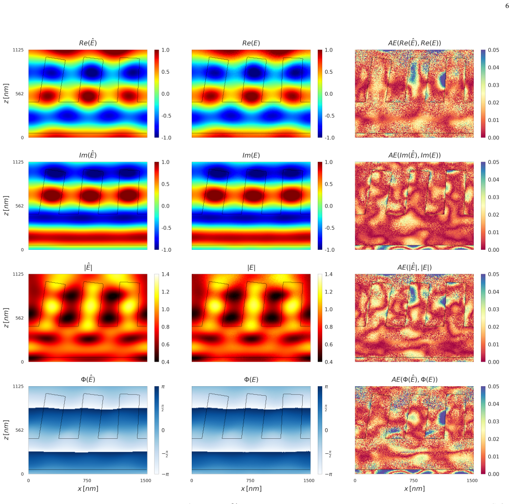
The authors state that, to the best of their knowledge, this is the first work to encode spatially varying PDE parameters into a physics-informed PointNet training framework. The network takes as input an unordered point cloud in which each point carries its spatial coordinate and the local permittivity $\varepsilon(x)$, and it outputs the real and imaginary parts of the electric field at every point (one scalar component $E_y$ in the 2D TE case; the vector field in 3D). Training minimizes a weighted sum of the Helmholtz residual inside the domain, a periodic boundary residual in the $x$- (and $y$-) direction, and an $L^2$ match to sparse reference solutions, with loss weights $\lambda_i=1$, $\lambda_b=1$, $\lambda_r=10$. On held-out domains in which only the three pillar inclination angles vary within $\pm 10^\circ$, the trained network generalizes to unseen material distributions; the paper's summary table reports near-field MAPE of $1.69\%\pm 0.43$ (2D SiO$_2$), $3.84\%\pm 0.13$ (3D SiO$_2$), and $10.72\%\pm 5.64$ (2D TiO$_2$), with 0th-order diffraction-efficiency APE of $1.95\%\pm 1.10$, $3.91\%\pm 4.18$, and $6.60\%\pm 3.37$ respectively. The authors frame this as evidence that a mesh-free network can learn the connection between material properties and electromagnetic response, not only geometry.

Load-bearing premise

The load-bearing premise is that a few hundred reference points plus the interior Helmholtz equation are enough to stop the top and bottom domain boundaries from reflecting light, because the stated non-reflective boundary condition never appears in the training loss.

Editorial extensions

If this is right

A single trained 2D network can predict the near-field and diffraction efficiency of a metasurface with new pillar tilts in about 100 ms of inference, after a roughly 2- to 4-hour training run, without rebuilding a mesh.
Spatially varying PDE parameters can be encoded as point-cloud features, so the method is not tied to a fixed material layout; the same network handles SiO2 and TiO2 metasurfaces by reading the local refractive index.
High material contrast is the main accuracy bottleneck: the TiO2-on-SiO2 case has roughly six times the near-field MAPE and more than three times the diffraction-efficiency APE of the SiO2 case.
Pointwise error grows with distance from the nearest reference point and falls with distance from material interfaces, so placing reference points near interfaces and boundaries is an effective way to improve accuracy.
Weak supervision from 224 reference points is enough in 2D; the experiments show that adding more reference points beyond that does not significantly lower the error.

Reading between the lines

Editorial extensions of the paper, not claims the author makes directly.

The paper does not test extrapolation in domain size; a direct extension would train on the 1125 nm tall domain and evaluate on taller or shorter truncations to expose whether the unenforced non-reflective boundary condition produces spurious reflections.
Because the permittivity is an input channel, the gradient of a predicted far-field metric with respect to per-point permittivity could be used for inverse design of material layouts, a route the paper leaves unexplored.
The same per-point parameter encoding should carry over to acoustic or elastic wave problems, where a spatially varying wave speed plays the role of $\varepsilon(x)$; this is an inference, not a paper claim.

Share X Bluesky LinkedIn Reddit HN

Editorial analysis

A structured set of objections, weighed in public.

Desk editor's note, referee report, and a circularity audit.

Desk Editor's Note

read the letter

Colleague,

The short version: this is a credible applied-ML paper with a clean novelty and honest experimental reporting, but it has a real boundary-condition gap and a clear 3D metric inconsistency. I'd send it to review, not reject it.

What's actually new: the per-point encoding of ε(x) into the PointNet input is a natural but clean extension of the Kashefi PIPN line, and the inclined-nanopillar metasurface application is new. The paper does a solid job of showing the method works on unseen inclination angles for fixed material systems, and the ablation studies (architecture, input scaling, reference point density) are useful. The training cost comparison to the mesh-based U-Net is genuinely informative.

Where it's soft: first, the non-reflective z-boundary condition stated in Sec. II-A never appears in the loss. Eq. (6) only enforces x-periodicity and the interior Helmholtz residual; the 224 interior reference points are the only constraint on the z-behavior. That makes the problem ill-posed as stated, and the network could be fitting the fixed-domain reference data rather than learning a radiation condition. The reported 1.69–10.72% MAPE may transfer within this fixed 1125 nm domain, but the paper's claim about modeling scattering is broader than that. This should be acknowledged and, ideally, the loss should include a z-boundary residual or the generalization claim should be narrowed. Second, the 3D numbers don't match: Table I gives MAPE 3.84±0.13 and APE 3.91±4.18, while the Sec. IV Case II text gives 3.04±0.09 and 1.12±0.28 for the same D_v. That's a reporting error that needs fixing. Third, the abstract's 'varying refractive indices' overstates what is demonstrated: each network is trained on a single material system (SiO2 or TiO2), so the model does not generalize across materials within one network.

The physics residual and RCWA reference data are external, so the circularity burden is low. The central idea holds up as a surrogate, not as a solver that learns radiation conditions. For the fixed-geometry, fixed-wavelength surrogate use case, the paper is a reasonable contribution.

Recommendation: accept for peer review with requests for the 3D number reconciliation, clarification of the z-boundary enforcement (or a narrowed generalization claim), and a code/data release statement. It's a useful paper for the ML-for-optics audience, and a good referee can get it into shape.

Referee Report

3 major / 2 minor

Summary. The manuscript presents a Physics-Informed PointNet (PIPN) that takes point clouds with spatial coordinates and local permittivity as input and predicts the electric field in all-dielectric metasurfaces with inclined nanopillars. The network is trained with a loss combining the Helmholtz residual, a periodic boundary residual, and sparse reference data from RCWA simulations. Three cases are tested: 2D SiO2, 3D SiO2, and 2D TiO2-on-SiO2, with varying pillar inclination angles. The reported near-field MAPEs are 1.69%, 3.84% (Table I) or 3.04% (text), and 10.72% for the three cases, with corresponding diffraction efficiency APEs. The central claim is that this is the first PIPN that encodes spatially varying PDE parameters and that the trained network generalizes to unseen inclination angles.

Significance. The method is potentially significant as a mesh-free, weakly supervised surrogate for optical metasurface simulation, with modest training costs (hours on a single GPU) and very fast inference. The use of external RCWA reference solutions and an independent Helmholtz residual is a credible validation strategy. However, the missing implementation of the z-direction radiation condition and the internal inconsistency in the 3D metrics need to be resolved before the claims can be accepted.

major comments (3)

[Sec. III-B, Eq. (6)] The boundary residual R_b enforces only the periodic conditions on the lateral boundaries. The non-reflective condition in z stated in Sec. II-A has no corresponding term in the loss, so the training objective does not correspond to a well-posed scattering problem. This is load-bearing because the claim is that the network learns the connection between material properties and electromagnetic response; without a radiation condition, the Helmholtz residual and reference loss may be satisfied by superpositions of spurious reflected waves that vanish at the reference points. The authors should add a boundary term for the z-faces (e.g., a first-order absorbing condition) or provide an experiment showing that predictions on a taller or shorter domain with the same trained network remain accurate; the current fixed domain of 1125 nm does not rule out the interpolation interpretation.
[Table I and Sec. IV, Case II] The same 3D SiO2 test set D_v is reported with near-field MAPE 3.84±0.13% and APE 3.91±4.18% in Table I, but with MAPE 3.04±0.09% and APE 1.12±0.28% in the text. This inconsistency is not a presentation typo; it concerns the central numerical result for the 3D case and must be resolved before publication.
[Abstract and Sec. II-B / IV] The claim of modeling "varying refractive indices" is not supported by the experiments. Each case has a fixed refractive index contrast (SiO2 or TiO2 on SiO2); only the inclination angles vary within a dataset. No experiment varies n continuously or tests n values unseen during training, so the assertion in the abstract that the method handles datasets "generated with varying refractive indices" overstates the demonstrated scope. Either add such an experiment (e.g., train on a range of n2 values and test on held-out n2) or rephrase the claim to say the framework can encode different fixed material configurations.

minor comments (2)

[Sec. III-C] The phrase "Asineactivation function" appears to contain a typo and should read "A sine activation function"; similarly, "traianble parameters" in Sec. IV, Case II, should be "trainable parameters".
[Sec. III-B, Eq. (6)] The definition of R_b is written explicitly for the 2D case only; the extension to 3D periodic boundaries in y is not specified, which makes the implementation of Case II ambiguous.

Circularity Check

1 steps flagged · score 4.0 of 10

Test-set hyperparameter selection makes the reported accuracy partly an input to the evaluation; the central physics-learning claim remains independent.

fitted input called prediction [Appendix A, Appendix C, Sec. IV (Table I)]
"Fig. 7 shows the near-fieldMAPEdistribution over all testing domains when the input coordinates and wavelength are scaled by different constants. The best results are achieved with a scaling factor around 21 (note the non-uniformx-axis). ... Results improve until N_r=224, when a near-fieldMAPEof1.88%is obtained; after that, the mean MAPEdoes not change significantly."

The input scaling factor and point-cloud sizes are selected by minimizing the near-field MAPE on the 50 testing domains. The same test MAPE is then reported in Table I and Sec. IV as the model's prediction accuracy. The reported generalization error is therefore the selection objective, not an independent out-of-sample estimate; the headline numbers are statistically forced by the test-set tuning and cannot be read as an unbiased evaluation of the learned material-to-response mapping.

full rationale

No step in the field-prediction chain is equivalent to its inputs: the Helmholtz residual is an independent PDE constraint, the reference loss enforces sparse RCWA data, and the test domains use inclination angles not seen in training. The central claim that spatially varying permittivity can be encoded and that the network generalizes across angles retains independent content. The main circularity concern is evaluation-only: hyperparameters (scaling factor ca. 21 and N_r/N_t) are selected by minimizing the very test MAPE later reported as the validation metric, so the numeric accuracy in Table I is inflated by selection on the test set. Separately, the non-reflective z-boundary stated in Sec. II-A is absent from the loss in Eq. (6), which is a well-posedness/generalization risk rather than a circularity; it does not raise the circularity score. Self-citations [26], [45] are used only for a computational comparison and are not load-bearing for the derivation.

Assumptions & free parameters 5 free parameters · 6 assumptions · 0 invented entities

The central result rests on a set of ML hyperparameters (scaling, loss weights, point counts, network size) that are tuned on the training set, and on domain assumptions about the physical model, the accuracy of the RCWA reference, and the sufficiency of sparse reference points. No new physical entities are introduced.

free parameters (5)

input coordinate scaling factor = 21
Appendix A: input x/z coordinates and wavelength are scaled by ~21 to achieve convergence; a tuned ML hyperparameter that the results depend on.
loss weights (λ_i, λ_b, λ_r) = 1, 1, 10
Sec. III-C: weighting factors set to 1, 1, 10, taken from prior studies; the central loss balance is sensitive to these values.
point cloud sizes (N_i, N_b, N_r) = 1696, 128, 224 (2D); 3392, 256, 448 (3D)
Appendix C: optimal configuration by tuning; increasing N_r or N_t does not improve beyond these.
network size N_θ = 252k (2D), 448k (3D)
Appendix B: architecture sizes selected based on error/compute tradeoff.
learning rate schedule = 1e-3 to 8e-5, polynomial decay 4.5
Sec. III-C: optimizer hyperparameters chosen by the authors.

assumptions (6)

domain assumption The time-harmonic Maxwell equations reduce to the vector or scalar Helmholtz equation for linear, isotropic, non-magnetic, lossless media with no free currents.
Sec. II-A, Eq. (1)-(2); the physical model is assumed valid for the all-dielectric metasurfaces considered.
domain assumption The reference solutions computed by the rigorous coupled-wave analysis solver are accurate ground truth.
Sec. II-B; the RCWA/waveguide method is trusted for both training labels and evaluation; the paper provides no independent experimental validation.
domain assumption The PointNet architecture with a symmetric max-pooling aggregation is sufficient to represent the mapping from per-point permittivity and geometry to the electric field.
Sec. III-A; the expressiveness of the architecture is assumed, not proven; Appendix B only tunes layer types and sizes.
domain assumption The sparse reference points disambiguate the trivial zero solution of the source-free Helmholtz equation.
Sec. II-A: the paper adds reference points explicitly because the PDE alone admits E=0 everywhere.
domain assumption The domain is exactly periodic in x (and y in 3D) with period 500 nm, and the incident plane wave is at normal incidence so the total field is periodic.
Sec. II-B: three unit cells are simulated; the periodic boundary residual in Eq. (6) enforces this.
ad hoc to paper The non-reflective boundary condition in z is implicitly satisfied by the reference points and the local nature of the solution.
Sec. II-A states the condition, but Sec. III-B does not include a corresponding residual loss; the paper assumes learning will handle it.

how reviews work

0 comments

Cite this review

Pith. "Pith review of Physics-Informed PointNets for Modeling Electromagnetic Scattering from All-Dielectric Metasurfaces with Inclined Nanopillars." pith.science (2026). https://pith.science/paper/BU2QRUK7

@misc{pith2026250723119,
  author       = {Pith},
  title        = {Pith review of: Physics-Informed PointNets for Modeling Electromagnetic Scattering from All-Dielectric Metasurfaces with Inclined Nanopillars},
  year         = {2026},
  howpublished = {\url{https://pith.science/paper/BU2QRUK7}},
  note         = {Machine review of arXiv:2507.23119}
}

read the original abstract

Metasurfaces are innovative planar optical structures capable of manipulating incident light properties. Accurate and computationally efficient modeling of such metasurfaces, particularly those with irregular geometries, remains a challenge for conventional solvers. In this work, we present a mesh-free Physics-Informed PointNet (PIPN) to model electromagnetic scattering from all-dielectric metasurfaces that feature spatially varying nanopillars. Our approach uses the PointNet architecture to directly encode spatially varying material properties into the Physics-Informed Machine Learning (PIML) framework. We demonstrate the generalization capability of our PIPN through evaluations on datasets; these datasets are generated with varying refractive indices representing common dielectric materials. Furthermore, the inclination angles are varied within each dataset, which represent expected manufacturing defects. Overall, our method provides a promising, mesh-free framework for accurate and efficient modeling of complex optical structures represented by irregular geometries.

Figures

Figures reproduced from arXiv: 2507.23119 by the authors.

**Figure 2.** A schematic of the PointNet architecture used in this work. The PointNet’s design leverages 1D convolutional kernels applied to each point individually [PITH_FULL_IMAGE:figures/full_fig_p004_2.png] view at source ↗

**Figure 3.** A representative approximate solution (near-field [PITH_FULL_IMAGE:figures/full_fig_p006_3.png] view at source ↗

Figures from the paper (6 more)

**Figure 4.** Figure 4: Representative solution for the 3D SiO2 Ey field at y ≈ 250 nm, with near-field MAPE = 4.04%. Metasurface geometry and material as indicated in Fig. 1b. future study for PIPN applications should be the generalization across diverse domain geometries, as opposed to the …

**Figure 5.** Figure 5: Representative solution for the 2D TiO2 dataset, with near-field MAPE = 10.01%. PIPN demonstrates significant computational advantages. Our approach can be trained on a NVIDIA Quadro P5000 GPU with 16 GB of VRAM in approximately 24 hours, whereas the mesh-based counter…

**Figure 7.** Figure 7: Relationship between the normalization factor (of the input spatial [PITH_FULL_IMAGE:figures/full_fig_p009_7.png]

**Figure 8.** Figure 8: Box plots of the test near-field MAPE versus the network size (Nθ) for three different variations of the PointNet architecture. The inset plot shows the relative training time (hours) versus the same network sizes. 252×103 parameters. In contrast, PointNetCNN consisten…

**Figure 10.** Figure 10: Correlation between the near-field MAE (averaged over the testing set Dv from Case I - 2D SiO2 Metasurface) at each test domain point and its minimum distance from the corresponding training reference points (green) and material interface (blue) [PITH_FULL_IMAGE:figu…

**Figure 9.** Figure 9: Box plots of the test near-field MAPE versus the number of reference points (Nr) used during training. The inset plot shows how varying the number of total points (Nt) used for training affects the near-field MAPE at a constant Nr = 224 [PITH_FULL_IMAGE:figures/full_f…

Discussion (0). Continue with ORCID to comment.

Reference graph

Works this paper leans on

45 extracted references · 39 canonical work pages

[1]

Optical metasurfaces: new generation building blocks for multi-functional optics,

D. Neshev and I. Aharonovich, “Optical metasurfaces: new generation building blocks for multi-functional optics,”Light: Science & Appli- cations, vol. 7, no. 1, p. 58, Aug. 2018, publisher: Nature Publishing Group

work page 2018
[2]

Roadmap for optical metasurfaces,

A. I. Kuznetsov, M. L. Brongersma, J. Yao, M. K. Chen, U. Levy, D. P. Tsai, N. I. Zheludev, A. Faraon, A. Arbabi, N. Yuet al., “Roadmap for optical metasurfaces,”ACS photonics, vol. 11, no. 3, pp. 816–865, 2024

work page 2024
[3]

Flat optics: controlling wavefronts with optical antenna metasurfaces,

N. Yu, P. Genevet, F. Aieta, M. A. Kats, R. Blanchard, G. Aoust, J.-P. Tetienne, Z. Gaburro, and F. Capasso, “Flat optics: controlling wavefronts with optical antenna metasurfaces,”IEEE Journal of Selected Topics in Quantum Electronics, vol. 19, no. 3, pp. 4 700 423–4 700 423, 2013. 11

work page 2013
[4]

Metasurface micro/nano-optical sensors: principles and applications,

J. Qin, S. Jiang, Z. Wang, X. Cheng, B. Li, Y . Shi, D. P. Tsai, A. Q. Liu, W. Huang, and W. Zhu, “Metasurface micro/nano-optical sensors: principles and applications,”ACS nano, vol. 16, no. 8, pp. 11 598– 11 618, 2022

work page 2022
[5]

Optical Metasurfaces for Biomedical Imaging and Sensing,

H. Kim, H. Yun, S. Jeong, S. Lee, E. Cho, and J. Rho, “Optical Metasurfaces for Biomedical Imaging and Sensing,”ACS Nano, vol. 19, no. 3, pp. 3085–3114, Jan. 2025, publisher: American Chemical Society

work page 2025
[6]

3D-Integrated metasurfaces for full-colour holography,

Y . Hu, X. Luo, Y . Chen, Q. Liu, X. Li, Y . Wang, N. Liu, and H. Duan, “3D-Integrated metasurfaces for full-colour holography,”Light: Science & Applications, vol. 8, no. 1, p. 86, Sep. 2019, publisher: Nature Publishing Group

work page 2019
[7]

Metasurfaces for multiplexed communi- cation,

S. Nie and I. F. Akyildiz, “Metasurfaces for multiplexed communi- cation,”Nature Electronics, vol. 4, no. 3, pp. 177–178, Mar. 2021, publisher: Nature Publishing Group

work page 2021
[8]

A programmable diffractive deep neural network based on a digital-coding metasurface array,

C. Liu, Q. Ma, Z. J. Luo, Q. R. Hong, Q. Xiao, H. C. Zhang, L. Miao, W. M. Yu, Q. Cheng, L. Li, and T. J. Cui, “A programmable diffractive deep neural network based on a digital-coding metasurface array,” Nature Electronics, vol. 5, no. 2, pp. 113–122, Feb. 2022, publisher: Nature Publishing Group

work page 2022

Show all 45 references

[9]

Time-Domain Finite-Difference and Finite-Element Methods for Maxwell Equations in Complex Media,

F. L. Teixeira, “Time-Domain Finite-Difference and Finite-Element Methods for Maxwell Equations in Complex Media,”IEEE Transactions on Antennas and Propagation, vol. 56, no. 8, pp. 2150–2166, Aug. 2008

2008
[10]

Fast near field simulation of optical and EUV masks using the waveguide method,

P. Evanschitzky and A. Erdmann, “Fast near field simulation of optical and EUV masks using the waveguide method,” inProceedings of the SPIE, Volume 6533, article id. 65330Y, vol. 6533, Feb. 2007, p. 65330Y , conference Name: 23rd European Mask and Lithography Conference ADS Bi...

2007
[11]

Large-scale photonic inverse design: computational challenges and breakthroughs,

C. Kang, C. Park, M. Lee, J. Kang, M. S. Jang, and H. Chung, “Large-scale photonic inverse design: computational challenges and breakthroughs,”Nanophotonics, vol. 13, no. 20, pp. 3765–3792, 2024

2024
[12]

Deep Convolutional Neural Networks to Predict Mutual Coupling Effects in Metasurfaces,

S. An, B. Zheng, M. Y . Shalaginov, H. Tang, H. Li, L. Zhou, Y . Dong, M. Haerinia, A. M. Agarwal, C. Rivero-Baleine, M. Kang, K. A. Richardson, T. Gu, J. Hu, C. Fowler, and H. Zhang, “Deep Convolutional Neural Networks to Predict Mutual Coupling Effects in Metasurfaces,” Adva...

2022
[13]

PISC-Net: A Comprehensive Neural Network Framework for Predicting Metasurface Infrared Emission Spec- tra,

C. Li, J. Chen, Q. Lin, and Y . Han, “PISC-Net: A Comprehensive Neural Network Framework for Predicting Metasurface Infrared Emission Spec- tra,”ACS Applied Materials & Interfaces, vol. 16, no. 32, pp. 42 816– 42 827, Aug. 2024, publisher: American Chemical Society

2024
[14]

Scientific Machine Learning Through Physics–Informed Neural Networks: Where we are and What’s Next,

S. Cuomo, V . S. Di Cola, F. Giampaolo, G. Rozza, M. Raissi, and F. Piccialli, “Scientific Machine Learning Through Physics–Informed Neural Networks: Where we are and What’s Next,”Journal of Scientific Computing, vol. 92, no. 3, p. 88, Jul. 2022

2022
[15]

Physics Informed Deep Learning (Part II): Data-driven Discovery of Nonlinear Partial Differential Equations,

M. Raissi, P. Perdikaris, and G. E. Karniadakis, “Physics Informed Deep Learning (Part II): Data-driven Discovery of Nonlinear Partial Differential Equations,” Nov. 2017, arXiv:1711.10566 [cs]

2017 arXiv
[16]

From PINNs to PIKANs: recent advances in physics-informed machine learning,

J. D. Toscano, V . Oommen, A. J. Varghese, Z. Zou, N. Ahmadi Daryak- enari, C. Wu, and G. E. Karniadakis, “From PINNs to PIKANs: recent advances in physics-informed machine learning,”Machine Learning for Computational Science and Engineering, vol. 1, no. 1, p. 15, Mar. 2025

2025
[17]

Physics-Informed Neural Network Inte- grating PointNet-Based Adaptive Refinement for Investigating Crack Propagation in Industrial Applications,

J. Tu, C. Liu, and P. Qi, “Physics-Informed Neural Network Inte- grating PointNet-Based Adaptive Refinement for Investigating Crack Propagation in Industrial Applications,”IEEE Transactions on Industrial Informatics, vol. 19, no. 2, pp. 2210–2218, Feb. 2023

2023
[18]

Physics- Informed Machine Learning for Industrial Reliability and Safety Engi- neering: A Review and Perspective,

D. H. Nguyen, T. H. Nguyen, K. D. Tran, and K. P. Tran, “Physics- Informed Machine Learning for Industrial Reliability and Safety Engi- neering: A Review and Perspective,” inArtificial Intelligence for Safety and Reliability Engineering: Methods, Applications, and Challenges, ...

2024
[19]

Loss landscape en- gineering via Data Regulation on PINNs,

V . Gopakumar, S. Pamela, and D. Samaddar, “Loss landscape en- gineering via Data Regulation on PINNs,”Machine Learning with Applications, vol. 12, p. 100464, Jun. 2023

2023
[20]

An Expert’s Guide to Training Physics-informed Neural Networks,

S. Wang, S. Sankaran, H. Wang, and P. Perdikaris, “An Expert’s Guide to Training Physics-informed Neural Networks,” Aug. 2023, arXiv:2308.08468 [cs]

2023 arXiv
[21]

Understanding and Mitigating Gradient Flow Pathologies in Physics-Informed Neural Networks,

S. Wang, Y . Teng, and P. Perdikaris, “Understanding and Mitigating Gradient Flow Pathologies in Physics-Informed Neural Networks,”SIAM Journal on Scientific Computing, vol. 43, no. 5, pp. A3055–A3081, Jan. 2021, publisher: Society for Industrial and Applied Mathematics

2021
[22]

Maxwellnet: Physics-driven deep neural network training based on maxwell’s equations,

J. Lim and D. Psaltis, “Maxwellnet: Physics-driven deep neural network training based on maxwell’s equations,”APL Photonics, vol. 7, no. 1, p. 011301, 01 2022

2022
[23]

Physics- informed deep model for fast time-domain electromagnetic simula- tion and inversion,

H. Liu, Y . Fan, F. Ding, L. Du, J. Zhao, C. Sun, and H. Zhou, “Physics- informed deep model for fast time-domain electromagnetic simula- tion and inversion,”IEEE Transactions on Antennas and Propagation, vol. 72, no. 10, pp. 7807–7820, 2024

2024
[24]

Multi-receptive-field physics-informed neural network for complex electromagnetic media,

Y . Wang and S. Zhang, “Multi-receptive-field physics-informed neural network for complex electromagnetic media,”Opt. Mater. Express, vol. 14, no. 11, pp. 2740–2754, Nov 2024

2024
[25]

Inverse Design for Integrated Photonics Using Deep Neural Network,

K. Kojima, T. Koike-Akino, Y . Tang, and Y . Wang, “Inverse Design for Integrated Photonics Using Deep Neural Network,” inIntegrated Nanophotonics: Platforms, Devices, and Applications. Wiley, 2023, pp. 209–243

2023
[26]

3D EUV mask simulator based on physics-informed neural networks: effects of polarization and illumination,

V . Medvedev, A. Erdmann, and A. Rosskopf, “3D EUV mask simulator based on physics-informed neural networks: effects of polarization and illumination,” inComputational Optics 2024, vol. 13023, International Society for Optics and Photonics. SPIE, 2024, p. 1302304

2024
[27]

3D mask simulation and lithographic imaging using physics-informed neural networks,

V . Medvedev, A. Erdmann, and A. Rosskopf, “3D mask simulation and lithographic imaging using physics-informed neural networks,” in Optical and EUV Nanolithography XXXVII, vol. 12953. SPIE, Apr. 2024, pp. 208–224

2024
[28]

Physics-informed deep learning for 3D modeling of light diffraction from optical metasurfaces,

V . Medvedev, A. Erdmann, and A. Rosskopf, “Physics-informed deep learning for 3D modeling of light diffraction from optical metasurfaces,” Opt. Express, vol. 33, no. 1, pp. 1371–1384, Jan 2025

2025
[29]

The Helmholtz equation in heterogeneous media: A priori bounds, well-posedness, and resonances,

I. Graham, O. Pembery, and E. Spence, “The Helmholtz equation in heterogeneous media: A priori bounds, well-posedness, and resonances,” Journal of Differential Equations, vol. 266, no. 6, pp. 2869–2923, Mar. 2019

2019
[30]

MaxwellNet: Physics-driven deep neural network training based on Maxwell’s equations,

J. Lim and D. Psaltis, “MaxwellNet: Physics-driven deep neural network training based on Maxwell’s equations,”APL Photonics, vol. 7, no. 1, p. 011301, Jan. 2022

2022
[31]

PointNet: A 3D Convolu- tional Neural Network for real-time object class recognition,

A. Garcia-Garcia, F. Gomez-Donoso, J. Garcia-Rodriguez, S. Orts- Escolano, M. Cazorla, and J. Azorin-Lopez, “PointNet: A 3D Convolu- tional Neural Network for real-time object class recognition,” in2016 International Joint Conference on Neural Networks (IJCNN), Jul. 2016, pp. ...

2016
[32]

PointNet++: Deep Hierarchical Feature Learning on Point Sets in a Metric Space,

C. R. Qi, L. Yi, H. Su, and L. J. Guibas, “PointNet++: Deep Hierarchical Feature Learning on Point Sets in a Metric Space,” inAdvances in Neural Information Processing Systems, vol. 30. Curran Associates, Inc., 2017

2017
[33]

Physics-informed PointNet: A deep learning solver for steady-state incompressible flows and thermal fields on multiple sets of irregular geometries,

A. Kashefi and T. Mukerji, “Physics-informed PointNet: A deep learning solver for steady-state incompressible flows and thermal fields on multiple sets of irregular geometries,”Journal of Computational Physics, vol. 468, p. 111510, Nov. 2022

2022
[34]

Physics-informed PointNet: On how many irregular geometries can it solve an inverse problem simul- taneously? Application to linear elasticity,

A. Kashefi, L. J. Guibas, and T. Mukerji, “Physics-informed PointNet: On how many irregular geometries can it solve an inverse problem simul- taneously? Application to linear elasticity,” Sep. 2023, arXiv:2303.13634 [cs]

2023 arXiv
[35]

Physics-informed pointnet: A deep learning solver for steady-state incompressible flows and thermal fields on multiple sets of irregular geometries,

A. Kashefi and T. Mukerji, “Physics-informed pointnet: A deep learning solver for steady-state incompressible flows and thermal fields on multiple sets of irregular geometries,”J. Comput. Phys., vol. 468, p. 111510, 2022

2022
[36]

KAN: Kolmogorov-Arnold Networks,

Z. Liu, Y . Wang, S. Vaidya, F. Ruehle, J. Halverson, M. Solja ˇci´c, T. Y . Hou, and M. Tegmark, “KAN: Kolmogorov-Arnold Networks,” Jun. 2024, arXiv:2404.19756 [cond-mat, stat]

2024 arXiv
[37]

A physics-informed deep convolutional neural network for simulating and predicting transient darcy flows in heterogeneous reservoirs without labeled data,

Z. Zhang, “A physics-informed deep convolutional neural network for simulating and predicting transient darcy flows in heterogeneous reservoirs without labeled data,”Journal of Petroleum Science and Engineering, vol. 211, p. 110179, 2022

2022
[38]

Adam: A Method for Stochastic Optimization,

D. P. Kingma and J. Ba, “Adam: A Method for Stochastic Optimization,” Jan. 2017, arXiv:1412.6980 [cs]

2017 arXiv
[39]

Prediction of fluid flow in porous media by sparse observations and physics-informed PointNet,

A. Kashefi and T. Mukerji, “Prediction of fluid flow in porous media by sparse observations and physics-informed PointNet,”Neural Networks, vol. 167, pp. 80–91, Oct. 2023

2023
[40]

Understanding the difficulty of training deep feedforward neural networks,

X. Glorot and Y . Bengio, “Understanding the difficulty of training deep feedforward neural networks,” inProceedings of the Thirteenth International Conference on Artificial Intelligence and Statistics. JMLR Workshop and Conference Proceedings, Mar. 2010, pp. 249–256, iSSN: 1938-7228

2010
[41]

On the spectral bias of neural networks,

N. Rahaman, A. Baratin, D. Arpit, F. Draxler, M. Lin, F. Hamprecht, Y . Bengio, and A. Courville, “On the spectral bias of neural networks,” in Proceedings of the 36th International Conference on Machine Learning, ser. Proceedings of Machine Learning Research, K. Chaudhuri and...

2019
[42]

A comprehensive study of non-adaptive and residual-based adaptive sampling for physics- informed neural networks,

C. Wu, M. Zhu, Q. Tan, Y . Kartha, and L. Lu, “A comprehensive study of non-adaptive and residual-based adaptive sampling for physics- informed neural networks,”Computer Methods in Applied Mechanics and Engineering, vol. 403, p. 115671, Jan. 2023

2023
[43]

FourierKAN outperforms MLP on Text Classification Head Fine-tuning,

A. A. Imran and M. F. Ishmam, “FourierKAN outperforms MLP on Text Classification Head Fine-tuning,” Sep. 2024, arXiv:2408.08803 [cs]

2024 arXiv
[44]

Kolmogorov-Arnold Networks are Radial Basis Function Net- works,

Z. Li, “Kolmogorov-Arnold Networks are Radial Basis Function Net- works,” May 2024, arXiv:2405.06721 [cs]. 12

2024 arXiv
[45]

Physics-informed deep learning for 3D modeling of light diffraction from optical metasurfaces,

V . Medvedev, A. Erdmann, and A. Rosskopf, “Physics-informed deep learning for 3D modeling of light diffraction from optical metasurfaces,” Optics Express, vol. 33, no. 1, p. 1371, Jan. 2025. Leon Armbrusterreceived his MSc in Applied and Computational Mathematics from Friedri...

2025

Pith tools

Reviewed August 6, 2026 · model on record in the stance chip above.

[1] [1]

Optical metasurfaces: new generation building blocks for multi-functional optics,

D. Neshev and I. Aharonovich, “Optical metasurfaces: new generation building blocks for multi-functional optics,”Light: Science & Appli- cations, vol. 7, no. 1, p. 58, Aug. 2018, publisher: Nature Publishing Group

work page 2018

[2] [2]

Roadmap for optical metasurfaces,

A. I. Kuznetsov, M. L. Brongersma, J. Yao, M. K. Chen, U. Levy, D. P. Tsai, N. I. Zheludev, A. Faraon, A. Arbabi, N. Yuet al., “Roadmap for optical metasurfaces,”ACS photonics, vol. 11, no. 3, pp. 816–865, 2024

work page 2024

[3] [3]

Flat optics: controlling wavefronts with optical antenna metasurfaces,

N. Yu, P. Genevet, F. Aieta, M. A. Kats, R. Blanchard, G. Aoust, J.-P. Tetienne, Z. Gaburro, and F. Capasso, “Flat optics: controlling wavefronts with optical antenna metasurfaces,”IEEE Journal of Selected Topics in Quantum Electronics, vol. 19, no. 3, pp. 4 700 423–4 700 423, 2013. 11

work page 2013

[4] [4]

Metasurface micro/nano-optical sensors: principles and applications,

J. Qin, S. Jiang, Z. Wang, X. Cheng, B. Li, Y . Shi, D. P. Tsai, A. Q. Liu, W. Huang, and W. Zhu, “Metasurface micro/nano-optical sensors: principles and applications,”ACS nano, vol. 16, no. 8, pp. 11 598– 11 618, 2022

work page 2022

[5] [5]

Optical Metasurfaces for Biomedical Imaging and Sensing,

H. Kim, H. Yun, S. Jeong, S. Lee, E. Cho, and J. Rho, “Optical Metasurfaces for Biomedical Imaging and Sensing,”ACS Nano, vol. 19, no. 3, pp. 3085–3114, Jan. 2025, publisher: American Chemical Society

work page 2025

[6] [6]

3D-Integrated metasurfaces for full-colour holography,

Y . Hu, X. Luo, Y . Chen, Q. Liu, X. Li, Y . Wang, N. Liu, and H. Duan, “3D-Integrated metasurfaces for full-colour holography,”Light: Science & Applications, vol. 8, no. 1, p. 86, Sep. 2019, publisher: Nature Publishing Group

work page 2019

[7] [7]

Metasurfaces for multiplexed communi- cation,

S. Nie and I. F. Akyildiz, “Metasurfaces for multiplexed communi- cation,”Nature Electronics, vol. 4, no. 3, pp. 177–178, Mar. 2021, publisher: Nature Publishing Group

work page 2021

[8] [8]

A programmable diffractive deep neural network based on a digital-coding metasurface array,

C. Liu, Q. Ma, Z. J. Luo, Q. R. Hong, Q. Xiao, H. C. Zhang, L. Miao, W. M. Yu, Q. Cheng, L. Li, and T. J. Cui, “A programmable diffractive deep neural network based on a digital-coding metasurface array,” Nature Electronics, vol. 5, no. 2, pp. 113–122, Feb. 2022, publisher: Nature Publishing Group

work page 2022