REVIEW 2 major objections 208 references
GINKAKU reduces differences in nonlinear power spectra across N-body codes to below 1 percent by tuning TreePM accuracy parameters and linear-response neutrino terms.
Reviewed by Pith at T0; open to challenge. T0 means a machine referee read the full paper against a public rubric. the ladder, T0–T4 →
T0 review · grok-4.3
2026-06-29 10:51 UTC pith:C4YQ4JHG
load-bearing objection GINKAKU is a new TreePM code on FDPS for controlled DQ2 ensembles with neutrinos and clustering DE, showing ~1% code-to-code P(k) agreement after tuning. the 2 major comments →
GINKAKU: Scalable Cosmological Structure Formation Simulation Code and Post-processing Pipeline
The pith
A machine-rendered reading of the paper's core claim, the machinery that carries it, and where it could break.
Core claim
GINKAKU demonstrates that its TreePM solver plus linear-response treatment of massive-neutrino, radiation, and clustering-dark-energy perturbations in the N-body gauge produces nonlinear matter power spectra that agree with established codes to within about 1 percent once accuracy parameters are tuned, at modest extra cost, and that the same framework reproduces the expected scale-dependent growth signatures in production-scale runs.
What carries the argument
Linear-response treatment of external source terms (massive neutrinos, radiation, clustering dark energy) in the N-body gauge, coupled to a TreePM gravity solver on the FDPS framework.
Load-bearing premise
The linear-response treatment of external source terms remains accurate on subhorizon scales without requiring full nonlinear particle evolution for those components.
What would settle it
A side-by-side run on identical initial conditions in which the fiducial GINKAKU settings produce a nonlinear power spectrum differing by more than 1 percent from PKDGRAV3 or RAMSES across the relevant k-range would falsify the accuracy claim.
If this is right
- Ensemble production across multiple cosmological models with massive neutrinos and clustering dark energy becomes feasible while keeping power-spectrum errors below 1 percent.
- The post-processing pipeline reduces inter-resolution scatter in the halo mass function to about 1 percent and supplies halo-shape data for intrinsic-alignment statistics.
- A total matter power spectrum emulator can be constructed directly from the production runs.
- Scale-dependent growth signatures from neutrinos and dark energy appear in the nonlinear regime as expected.
Where Pith is reading between the lines
- If the linear-response approximation holds, other relativistic or early-universe components could be added at the linear level without full particle evolution.
- The controlled accuracy opens the possibility of running larger ensembles or higher-resolution boxes while staying within survey requirements for systematic error budgets.
- Direct comparison of the same initial conditions evolved in different gauges would test how much the N-body gauge choice affects the final 1 percent agreement.
Editorial analysis
A structured set of objections, weighed in public.
Referee Report
Summary. The manuscript introduces GINKAKU, a new cosmological N-body code built on the FDPS framework that couples a TreePM gravity solver with linear-response treatment (in the N-body gauge) of external source terms for massive neutrinos, radiation, and clustering dark energy. It reports internal convergence studies and cross-comparisons with GADGET, PKDGRAV3, and RAMSES on shared initial conditions, claiming that tuning internal accuracy parameters reduces code-to-code differences in the nonlinear power spectrum below the ~1% level, with a production-grade fiducial setting identified at modest cost. The code is applied to an initial set of Dark Quest II production runs (eight cosmological models, 3000^3 particles in boxes up to 4 h^{-1} Gpc) processed by a renewed post-processing pipeline that reduces inter-resolution halo mass function spread to ~1% and includes halo-shape measurements; the runs reproduce expected nonlinear signatures of massive neutrinos and clustering dark energy, with a total matter power spectrum emulator presented in an accompanying paper.
Significance. If the numerical control and post-processing claims hold, GINKAKU would provide a scalable platform for generating the large simulation ensembles needed for next-generation galaxy surveys, incorporating linear-response effects of massive neutrinos and clustering dark energy at controlled ~1% accuracy on power spectra and halo statistics.
major comments (2)
- [Abstract] Abstract: the central validation claim rests on cross-code agreement at <1% in nonlinear P(k) under a shared linear-response treatment for neutrinos/DE/radiation; this tests numerical consistency of the TreePM solver and parameter tuning across implementations but does not test the accuracy of the linear-response approximation itself on subhorizon scales (k ≳ 0.1 h Mpc^{-1}) where nonlinear evolution of those components could matter. No quantitative benchmark against a full particle-based neutrino reference is reported.
- [Abstract] Abstract and validation description: the statement that the DQ2 runs 'reproduce the expected nonlinear signatures' is presented as a qualitative consistency check rather than a quantitative test of the linear-response treatment's validity; this leaves the physical accuracy of the approximation unquantified for the production runs.
Simulated Author's Rebuttal
We thank the referee for the careful review and constructive comments on the scope of our validation. We respond point-by-point below and will revise the abstract and validation sections to clarify that the presented tests address numerical consistency of the TreePM implementation under the linear-response treatment, rather than the physical accuracy of the approximation itself.
read point-by-point responses
-
Referee: [Abstract] Abstract: the central validation claim rests on cross-code agreement at <1% in nonlinear P(k) under a shared linear-response treatment for neutrinos/DE/radiation; this tests numerical consistency of the TreePM solver and parameter tuning across implementations but does not test the accuracy of the linear-response approximation itself on subhorizon scales (k ≳ 0.1 h Mpc^{-1}) where nonlinear evolution of those components could matter. No quantitative benchmark against a full particle-based neutrino reference is reported.
Authors: We agree that the cross-code comparisons (with GADGET, PKDGRAV3, and RAMSES) under the shared linear-response treatment validate numerical consistency and parameter tuning of the TreePM solver, but do not test the physical accuracy of the linear-response approximation against a fully nonlinear treatment of neutrinos or clustering dark energy on subhorizon scales. No quantitative benchmark against a full particle-based neutrino reference is included, as this manuscript focuses on code implementation, internal convergence, and controlled production for the DQ2 campaign. We will revise the abstract to explicitly state the scope of the validation. revision: yes
-
Referee: [Abstract] Abstract and validation description: the statement that the DQ2 runs 'reproduce the expected nonlinear signatures' is presented as a qualitative consistency check rather than a quantitative test of the linear-response treatment's validity; this leaves the physical accuracy of the approximation unquantified for the production runs.
Authors: The statement that the DQ2 runs reproduce expected nonlinear signatures is intended as a qualitative consistency check demonstrating that the code produces physically plausible scale-dependent effects (e.g., neutrino suppression). It is not presented as a quantitative test of the linear-response approximation's validity. We will revise the abstract and validation description to make this distinction clearer and to note that the physical accuracy relies on the established linear-response formalism. revision: yes
Circularity Check
No significant circularity in validation or design claims
full rationale
The paper introduces GINKAKU as a new N-body code using TreePM solver plus linear-response treatment for neutrinos/DE/radiation in N-body gauge, then validates via direct cross-comparisons against independent external codes (GADGET, PKDGRAV3, RAMSES) on shared initial conditions. The central empirical claim—that tuning internal accuracy parameters reduces code-to-code nonlinear P(k) differences below ~1%—is a measured outcome of those external benchmarks, not a fitted parameter renamed as prediction or a derivation that reduces to its own inputs by construction. No self-citation load-bearing steps, uniqueness theorems imported from the same authors, or ansatzes smuggled via prior work appear in the abstract or described content. The linear-response approximation is presented as a deliberate design choice whose physical accuracy on subhorizon scales is not derived within the paper but taken as given for the production runs; the reported agreement tests numerical consistency across implementations rather than closing a self-referential loop. This is a standard code-validation manuscript with externally falsifiable benchmarks.
Axiom & Free-Parameter Ledger
free parameters (1)
- internal accuracy parameters
axioms (1)
- domain assumption Linear-response treatment of neutrinos, radiation, and clustering dark energy remains valid on subhorizon scales in N-body gauge
read the original abstract
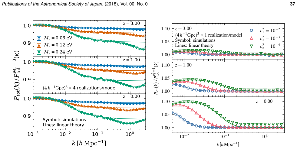
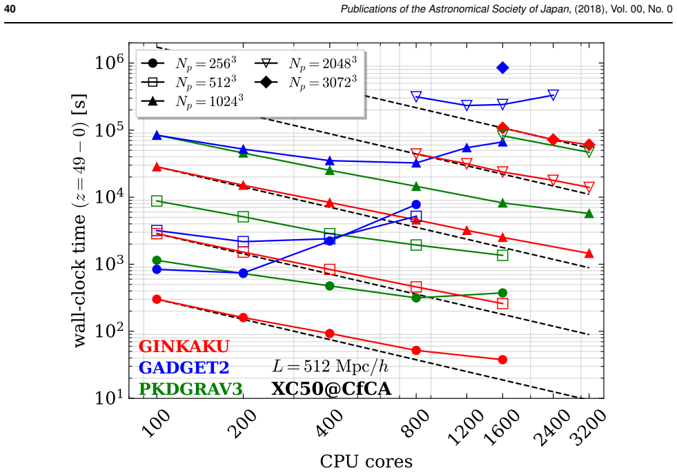
We introduce GINKAKU, a new cosmological $N$-body code developed for the Dark Quest II (DQ2) simulation campaign and designed for controlled ensemble production across the cosmological model space required by next-generation galaxy surveys, including massive neutrinos and clustering dark energy. Built on the FDPS framework, GINKAKU couples a TreePM gravity solver with a linear-response treatment of external source terms for components not evolved as $N$-body particles, formulated in the $N$-body gauge. This design incorporates massive-neutrino perturbations, general-relativistic corrections, early-time radiation perturbations, and dark-energy clustering with non-unit effective sound speed at the linear level, while preserving Newtonian particle dynamics on subhorizon scales. The code is validated through internal convergence studies and cross-comparisons with GADGET, PKDGRAV3, and RAMSES on shared initial conditions: code-to-code differences in the nonlinear power spectrum can be reduced below $\sim1\%$ level by tuning internal accuracy parameters, and we identify a production-grade fiducial setting achieving this control at modest cost. We apply GINKAKU to an initial set of DQ2 production runs -- eight cosmological models with $3,000^3$ particles in boxes up to $4\,h^{-1}\mathrm{Gpc}$ -- processed by a renewed post-processing pipeline that reduces the inter-resolution spread of the halo mass function to $\sim 1\%$ and includes halo-shape measurements for intrinsic-alignment statistics. The scale-dependent-growth cosmologies reproduce the expected nonlinear signatures of massive neutrinos and clustering dark energy, demonstrating suitability for emulator-scale production. A total matter power spectrum emulator from these runs is presented in an accompanying paper. (abridged)
Figures




Reference graph
Works this paper leans on
-
[1]
Abbott, T. M. C., Aguena, M., Alarcon, A., et al. 2022, Phys. Rev. D, 105, 023520 Abdul Karim, M., Aguilar, J., Ahlen, S., et al. 2025, Phys. Rev. D, 112, 083515
2022
-
[2]
G., Aguilar, J., Ahlen, S., et al
Adame, A. G., Aguilar, J., Ahlen, S., et al. 2025, JCAP, 2025, 021
2025
-
[3]
2017, MNRAS, 470, 303
Adamek, J., Brandbyge, J., Fidler, C., et al. 2017, MNRAS, 470, 303
2017
-
[4]
2016, JCAP, 2016, 053
Adamek, J., Daverio, D., Durrer, R., & Kunz, M. 2016, JCAP, 2016, 053
2016
-
[5]
B., Feldman, H
Agarwal, S., Abdalla, F. B., Feldman, H. A., Lahav, O., & Thomas, S. A. 2012, MNRAS, 424, 1409 —. 2014, MNRAS, 439, 2102
2012
-
[6]
2020, JCAP, 2020, 047
Aiola, S., Calabrese, E., Maurin, L., et al. 2020, JCAP, 2020, 047
2020
-
[7]
2021, Physical Review D, 103
Akitsu, K., Kurita, T., Nishimichi, T., Takada, M., & Tanaka, S. 2021, Physical Review D, 103
2021
-
[8]
2021, Phys
Alam, S., Aubert, M., Avila, S., et al. 2021, Phys. Rev. D, 103, 083533 Ali-Ha¨ımoud, Y ., & Bird, S. 2013, MNRAS, 428, 3375
2021
-
[9]
A., et al
Amon, A., Gruen, D., Troxel, M. A., et al. 2022, Phys. Rev. D, 105, 023514
2022
-
[10]
E., Zennaro, M., Contreras, S., et al
Angulo, R. E., Zennaro, M., Contreras, S., et al. 2021, MNRAS, 507, 5869
2021
-
[11]
E., Contreras, S., et al
Aric`o, G., Angulo, R. E., Contreras, S., et al. 2021, MNRAS, 506, 4070
2021
-
[12]
2021, A&A, 645, A104
Asgari, M., Lin, C.-A., Joachimi, B., et al. 2021, A&A, 645, A104
2021
-
[13]
2020, JCAP, 2020, 034
Aviles, A., & Banerjee, A. 2020, JCAP, 2020, 034
2020
-
[14]
Bagla, J. S. 2002, Journal of Astrophysics and Astronomy, 23, 185
2002
-
[15]
2015, Physical Review D, 92
Baldauf, T., Mercolli, L., & Zaldarriaga, M. 2015, Physical Review D, 92
2015
-
[16]
2016, Journal of Cosmology and Astroparticle Physics, 2016, 017–017
Baldauf, T., Schaan, E., & Zaldarriaga, M. 2016, Journal of Cosmology and Astroparticle Physics, 2016, 017–017
2016
-
[17]
2018, JCAP, 2018, 028
Banerjee, A., Powell, D., Abel, T., & Villaescusa-Navarro, F. 2018, JCAP, 2018, 028
2018
-
[18]
1986, Nature, 324, 446
Barnes, J., & Hut, P. 1986, Nature, 324, 446
1986
-
[19]
S., Wechsler, R
Behroozi, P. S., Wechsler, R. H., & Wu, H.-Y . 2013, ApJ, 762, 109
2013
-
[20]
A., & Weinberg, D
Berlind, A. A., & Weinberg, D. H. 2002, ApJ, 575, 587
2002
-
[21]
2002, 46Publications of the Astronomical Society of Japan, (2018), Vol
Bernardeau, F., Colombi, S., Gazta ˜naga, E., & Scoccimarro, R. 2002, 46Publications of the Astronomical Society of Japan, (2018), Vol. 00, No. 0 Phys. Rep., 367, 1
2002
-
[22]
2018, MNRAS, 481, 1486
Bird, S., Ali-Ha¨ımoud, Y ., Feng, Y ., & Liu, J. 2018, MNRAS, 481, 1486
2018
-
[23]
Bird, S., Viel, M., & Haehnelt, M. G. 2012, MNRAS, 420, 2551
2012
-
[24]
Effects of Massive Neutrinos and Dynamical Dark Energy on the Cluster Mass Function
Biswas, R., Heitmann, K., Habib, S., et al. 2019, arXiv e-prints, arXiv:1901.10690
work page internal anchor Pith review Pith/arXiv arXiv 2019
-
[25]
2011, JCAP, 7, 034
Blas, D., Lesgourgues, J., & Tram, T. 2011, JCAP, 7, 034
2011
-
[26]
2020, ApJ, 901, 5
Bocquet, S., Heitmann, K., Habib, S., et al. 2020, ApJ, 901, 5
2020
-
[27]
R., Colombi, S., Hivon, E., & Juszkiewicz, R
Bouchet, F. R., Colombi, S., Hivon, E., & Juszkiewicz, R. 1995, Astronomy and Astrophysics, 296, 575
1995
-
[28]
R., Juszkiewicz, R., Colombi, S., & Pellat, R
Bouchet, F. R., Juszkiewicz, R., Colombi, S., & Pellat, R. 1992, The Astrophysical Journal Letters, 394, L5
1992
-
[29]
2009, JCAP, 2009, 002
Brandbyge, J., & Hannestad, S. 2009, JCAP, 2009, 002
2009
-
[30]
Brandbyge, J., Hannestad, S., Haugbølle, T., & Wong, Y . Y . Y . 2010, JCAP, 2010, 014
2010
-
[31]
2017, MNRAS, 466, L68
Brandbyge, J., Rampf, C., Tram, T., et al. 2017, MNRAS, 466, L68
2017
-
[32]
2021, JCAP, 2021, 013
Brando, G., Koyama, K., & Wands, D. 2021, JCAP, 2021, 013
2021
-
[33]
2022, ApJ, 938, 110
Brout, D., Scolnic, D., Popovic, B., et al. 2022, ApJ, 938, 110
2022
-
[34]
L., & Norman, M
Bryan, G. L., & Norman, M. L. 1998, ApJ, 495, 80
1998
-
[35]
K., Villaescusa-Navarro, F., & Viel, M
Castorina, E., Sefusatti, E., Sheth, R. K., Villaescusa-Navarro, F., & Viel, M. 2014, JCAP, 2014, 049
2014
-
[36]
2025, Science China Physics, Mechanics, and Astronomy, 68, 109513
Chen, Z., & Yu, Y . 2025, Science China Physics, Mechanics, and Astronomy, 68, 109513
2025
-
[37]
2025, Science China Physics, Mechanics, and Astronomy, 68, 289512
Chen, Z., Yu, Y ., Han, J., & Jing, Y . 2025, Science China Physics, Mechanics, and Astronomy, 68, 289512
2025
-
[38]
E., & Dvorkin, C
Chisari, N. E., & Dvorkin, C. 2013, Journal of Cosmology and Astroparticle Physics, 2013, 029–029
2013
-
[39]
E., & Zaldarriaga, M
Chisari, N. E., & Zaldarriaga, M. 2011, Phys. Rev. D, 83, 123505
2011
-
[40]
J., Peacock, J
Cole, S., Percival, W. J., Peacock, J. A., et al. 2005, MNRAS, 362, 505
2005
-
[41]
H., & Kravtsov, A
Conroy, C., Wechsler, R. H., & Kravtsov, A. V . 2006, ApJ, 647, 201
2006
-
[42]
2002, Phys
Cooray, A., & Sheth, R. 2002, Phys. Rep., 372, 1
2002
-
[43]
2013, JCAP, 2013, 012
Costanzi, M., Villaescusa-Navarro, F., Viel, M., et al. 2013, JCAP, 2013, 012
2013
-
[44]
J., & Gazta ˜naga, E
Crocce, M., Fosalba, P., Castander, F. J., & Gazta ˜naga, E. 2010, Mon. Not. Roy. Astron. Soc., 403, 1353
2010
-
[45]
2006, Mon
Crocce, M., Pueblas, S., & Scoccimarro, R. 2006, Mon. Not. Roy. Astron. Soc., 373, 369
2006
-
[46]
2006a, Phys
Crocce, M., & Scoccimarro, R. 2006a, Phys. Rev. D, 73, 063520 —. 2006b, Phys. Rev. D, 73, 063519 —. 2008, Phys. Rev. D, 77, 023533
2008
-
[47]
2019, JCAP, 2019, 013
Dakin, J., Hannestad, S., Tram, T., Knabenhans, M., & Stadel, J. 2019, JCAP, 2019, 013
2019
-
[48]
R., & Shirokov, A
Dalal, N., White, M., Bond, J. R., & Shirokov, A. 2008, ApJ, 687, 12
2008
-
[49]
2023, Phys
Dalal, R., Li, X., Nicola, A., et al. 2023, Phys. Rev. D, 108, 123519
2023
-
[50]
2000, Astrophys
Dehnen, W. 2000, Astrophys. J., 536, L39 —. 2002, J. Comput. Phys., 179, 27
2000
-
[51]
Dehnen, W., & Read, J. I. 2011, European Physical Journal Plus, 126, 55
2011
-
[52]
H., Tinker, J
DeRose, J., Wechsler, R. H., Tinker, J. L., et al. 2019, ApJ, 875, 69 DES Collaboration, Abbott, T. M. C., Acevedo, M., et al. 2024, ApJL, 973, L14
2019
-
[53]
2018, Phys
Desjacques, V ., Jeong, D., & Schmidt, F. 2018, Phys. Rep., 733, 1
2018
-
[54]
Diemer, B., & Kravtsov, A. V . 2014, ApJ, 789, 1
2014
-
[55]
G., Kotok, E
Doroshkevich, A. G., Kotok, E. V ., Poliudov, A. N., et al. 1980, MNRAS, 192, 321
1980
-
[56]
Dutcher, D., Balkenhol, L., Ade, P. A. R., et al. 2021, Phys. Rev. D, 104, 022003
2021
-
[57]
J., Zehavi, I., Hogg, D
Eisenstein, D. J., Zehavi, I., Hogg, D. W., et al. 2005, ApJ, 633, 560
2005
-
[58]
S., Jenkins, A., Li, B., & Pascoli, S
Elbers, W., Frenk, C. S., Jenkins, A., Li, B., & Pascoli, S. 2022, MNRAS, 516, 3821
2022
-
[59]
2006, in Proceedings of the 2006 ACM/IEEE conference on Supercomputing, SC ’06 (New York, NY , USA: Association for Computing Machinery), 188–es
Elsen, E., Houston, M., Vishal, V ., et al. 2006, in Proceedings of the 2006 ACM/IEEE conference on Supercomputing, SC ’06 (New York, NY , USA: Association for Computing Machinery), 188–es
2006
-
[60]
2025, PASJ, 77, 337 Euclid Collaboration, Knabenhans, M., Stadel, J., et al
Enomoto, Y ., Taruya, A., Tanaka, S., & Nishimichi, T. 2025, PASJ, 77, 337 Euclid Collaboration, Knabenhans, M., Stadel, J., et al. 2019, MNRAS, 484, 5509 —. 2021, MNRAS, 505, 2840 Euclid Collaboration, Castro, T., Fumagalli, A., et al. 2023, A&A, 671, A100
2025
-
[61]
Faltenbacher, A., & White, S. D. M. 2010, ApJ, 708, 469
2010
-
[62]
2015, Phys
Fidler, C., Rampf, C., Tram, T., et al. 2015, Phys. Rev. D, 92, 123517
2015
-
[63]
2016, JCAP, 2016, 031
Fidler, C., Tram, T., Rampf, C., et al. 2016, JCAP, 2016, 031
2016
-
[64]
C., Hoekstra, H., Joachimi, B., et al
Fortuna, M. C., Hoekstra, H., Joachimi, B., et al. 2021, MNRAS, 501, 2983
2021
-
[65]
Gao, L., Springel, V ., & White, S. D. M. 2005, MNRAS, 363, L66
2005
-
[66]
Gao, L., & White, S. D. M. 2007, MNRAS, 377, L5
2007
-
[67]
H., Eisenstein, D
Garrison, L. H., Eisenstein, D. J., Ferrer, D., Metchnik, M. V ., & Pinto, P. A. 2016, MNRAS, 461, 4125
2016
-
[68]
H., Eisenstein, D
Garrison, L. H., Eisenstein, D. J., Ferrer, D., et al. 2018, ApJS, 236, 43
2018
-
[69]
Greengard, L., & Rokhlin, V . 1987, J. Comput. Phys., 73, 325
1987
-
[70]
2007, Phys
Habib, S., Heitmann, K., Higdon, D., Nakhleh, C., & Williams, B. 2007, Phys. Rev. D, 76, 083503
2007
-
[71]
2016, New Astron., 42, 49
Habib, S., Pope, A., Finkel, H., et al. 2016, New Astron., 42, 49
2016
-
[72]
2009, in 2009 NASA/ESA Conference on Adaptive Hardware and Systems, 447– 452
Hamada, T., Benkrid, K., Nitadori, K., & Taiji, M. 2009, in 2009 NASA/ESA Conference on Adaptive Hardware and Systems, 447– 452
2009
-
[73]
2020, PASJ, 72, 16
Hamana, T., Shirasaki, M., Miyazaki, S., et al. 2020, PASJ, 72, 16
2020
-
[74]
Hamilton, A. J. S. 2000, MNRAS, 312, 257
2000
-
[75]
2019, MNRAS, 482, 1900
Han, J., Li, Y ., Jing, Y ., et al. 2019, MNRAS, 482, 1900
2019
-
[76]
E., Robertson, A., & McCarthy, I
Harvey, D., Chisari, N. E., Robertson, A., & McCarthy, I. G. 2021, Monthly Notices of the Royal Astronomical Society, 506, 441–451
2021
-
[77]
2019, JCAP, 2019, 011
Hassani, F., Adamek, J., Kunz, M., & Vernizzi, F. 2019, JCAP, 2019, 011
2019
-
[78]
2020, JCAP, 2020, 039
Hassani, F., L’Huillier, B., Shafieloo, A., Kunz, M., & Adamek, J. 2020, JCAP, 2020, 039
2020
-
[79]
2006, ApJL, 646, L1
Heitmann, K., Higdon, D., Nakhleh, C., & Habib, S. 2006, ApJL, 646, L1
2006
-
[80]
2009, ApJ, 705, 156
Heitmann, K., Higdon, D., White, M., et al. 2009, ApJ, 705, 156
2009
discussion (0)
Sign in with ORCID, Apple, or X to comment. Anyone can read and Pith papers without signing in.