REVIEW 4 major objections 5 minor 30 references
The paper claims that the intractable joint posterior of states and parameters can be approximated online by factorizing it into a parameter marginal and a state conditional, with a two-stage KL-minimization update that keeps total approxim
Reviewed by Pith at T0; open to challenge. T0 means a machine referee read the full paper against a public rubric. the ladder, T0–T4 →
T0 review · deepseek-v4-flash
2026-08-03 13:10 UTC pith:C5WTPCF4
load-bearing objection A solid extension of the authors' earlier two-stage idea, with real experimental breadth, but the main theorem does not cover the surrogate-trained networks actually used in Stage 2, and the paper should be more explicit about that. the 4 major comments →
Sequential Bayesian parameter-state estimation in dynamical systems with noisy and incomplete observations via a variational framework
The pith
A machine-rendered reading of the paper's core claim, the machinery that carries it, and where it could break.
Core claim
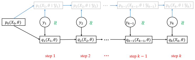
The central claim is that the Bayesian joint posterior p(X_k, θ | Y^k) can be approximated online with controlled error by the factorization q_k(X_k, θ) = ρ_k(X_k | θ) ν_k(θ), where ν_k is an arbitrary variational distribution over parameters and ρ_k is a conditional Gaussian with mean m_k(θ) and covariance C_k(θ). Rather than matching the intractable exact posterior directly, each step matches two 'online targets': ρ*_k, the conditional filter that would result from applying the exact prediction-update operators to the previous approximations, and ν*_k, the corresponding parameter posterior. The paper proves that the total-variation and Hellinger distances between the true joint posterior a
What carries the argument
The engine is the two-stage KL-minimization against online targets. The approximate joint posterior is written q_k(X_k, θ) = ρ_k(X_k|θ) ν_k(θ), and the online targets ρ*_k and ν*_k are what the exact filter recursions would produce if the previous approximations were used in place of the true conditional and parameter posteriors. Theorem 1 shows that tracking these targets tightly controls the distance to the true joint posterior. The state conditional ρ_k is represented as a Gaussian with mean m_k(θ) and covariance C_k(θ), implemented as time-invariant neural networks trained on target values provided by a Kalman filter or another Gaussian filter; in the high-dimensional experiment, an ense
Load-bearing premise
The practical error bound presumes that the neural networks trained in Stage 2 actually drive the expected KL divergences to small values; the theorem bounds the joint error only by those KL terms, and the paper does not prove that the trained networks achieve small KL—if the surrogate fitting is poor, the stated guarantee does not apply.
What would settle it
Take a linear system where the exact Kalman-filter posterior is computable, run FBOVI over many steps, and compare the true total-variation or Hellinger distance between the exact joint posterior and the approximation with the right-hand side of the paper's estimable bound, evaluated by Monte Carlo. If the observed error consistently exceeds the estimated bound, or stays small when the estimated per-step KL terms are large, then the stability theorem or the ELBO-based step in the proof has failed.
If this is right
- If the theorem is right, practitioners can choose any variational family for ν_k and any Gaussian filter for Stage 2, and the joint approximation error is still controlled by how well each step tracks its online target.
- Per-step computational cost stays bounded over time: only ν_k and the functions m_k(θ), C_k(θ) are passed forward, so historical data never needs to be replayed.
- For linear systems, the paper derives a bound that can be estimated from the algorithm's own outputs—m_i, C_i, ν_i, and ELBO values—giving a practical, checkable diagnostic of approximation accuracy.
- The every-step resampling variant lets the ensemble Kalman filter be used without carrying state particles forward, which is what allows the method to scale to a 51-dimensional discretized PDE system.
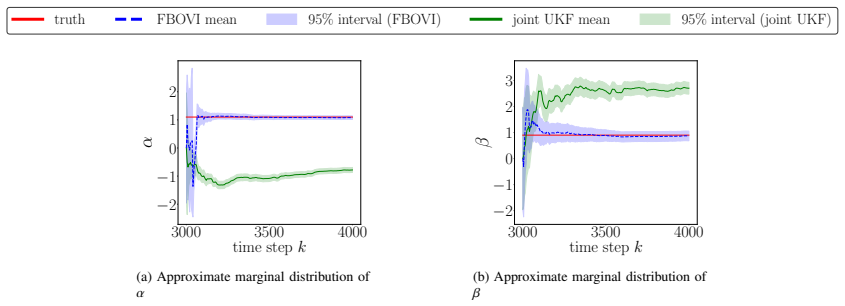
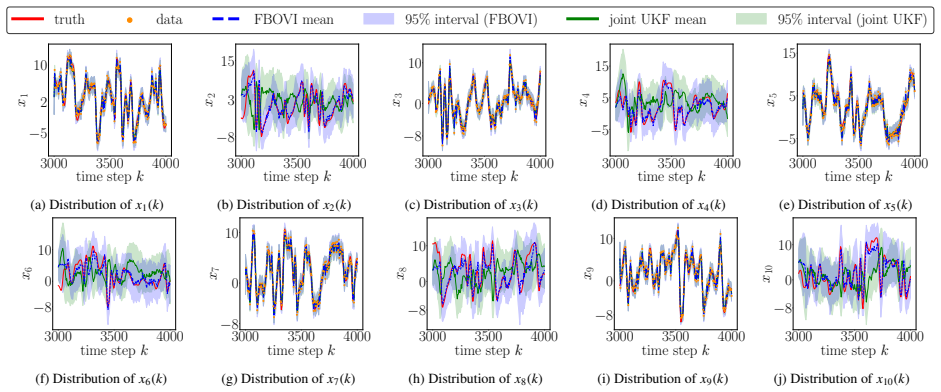
- Because the factorization is not mean-field—states remain conditioned on parameters—the marginal state distributions can be non-Gaussian even when the conditional filter is Gaussian, as shown in the chaotic-system experiments.
Where Pith is reading between the lines
- An extension the paper leaves implicit: the same two-stage KL structure could be run with a non-Gaussian ρ_k, for example a normalizing flow, provided the filtering step can supply target samples; the theorem only requires the KL terms, not Gaussianity.
- A practical diagnostic suggested by the estimable bound: monitor Monte Carlo estimates of the per-step KL terms and the ELBO; sustained drift would flag that the approximation has left the regime where the bound applies.
- The data-dependent constants in the bound involve inverse powers of the minimal measurement-noise determinant, implying that accuracy guarantees degrade when measurements are weakly informative or nearly collinear—a testable prediction about when the method can be trusted.
Editorial analysis
A structured set of objections, weighed in public.
Referee Report
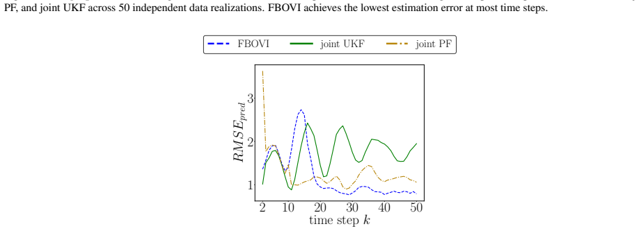
Summary. The paper proposes FBOVI, an online variational framework for joint state-parameter estimation in partially observed nonlinear dynamical systems. The approximate joint posterior is factorized as q_k(X_k, θ)=ρ_k(X_k|θ)ν_k(θ), with ν_k updated by maximizing an ELBO and ρ_k obtained by Gaussian filtering whose mean/covariance functions are represented by neural networks. The main theoretical contribution is Theorem 1, an upper bound on TV/Hellinger distance between the true posterior and q_k in terms of past KL divergences between the approximations and recursively defined online targets, and Theorem 2, an estimable version for linear systems. The framework is tested on a linear pendulum, a chaotic Lorenz-96 system, and a 51-dimensional convection-diffusion PDE, comparing with joint particle, unscented, and ensemble Kalman filters.
Significance. If the gap between the theoretical statement and the implemented algorithm were closed, this would be a useful contribution: the framework is modular, allows different Gaussian filters including the EnKF, and proposes an interpretable error bound that directly informs algorithmic choices. The numerical experiments are broad and show competitive accuracy, including robustness under model misspecification and high-dimensional state spaces. However, the advertised theoretical guarantee does not currently apply to the algorithm as implemented in the nonlinear/EnKF settings, and the proof of the central theorem is imported from an unpublished same-author preprint. These issues affect the central claim and should be resolved before acceptance.
major comments (4)
- [Sec. 3.2.2, Eqs. (25)-(26)] Theorem 1 bounds the joint posterior error by sums of E_{θ~ν_j}[KL(ρ_j‖ρ*_j)] and KL(ν_j‖ν*_j). Stage 1 targets the second KL, but Stage 2 does not minimize the first KL when the surrogate losses of Eq. (26) are used. Small MSE/Frobenius errors do not control the Gaussian KL: if C* is ill-conditioned or C has a small eigenvalue, KL contains log|C*|-log|C|+Tr(C*^{-1}C)+δ^T C*^{-1}δ, which can remain large even when ‖C-C*‖_F and ‖m-m*‖_2 are small. The theorem therefore does not transfer to the algorithm actually run in Section 4 unless the authors either train with the KL loss, prove that the surrogate losses bound the KL under explicit conditions, or verify in each experiment that the trained networks drive the KL terms small.
- [Sec. 3.1.2 Eqs. (15)-(18) vs. Eq. (9)] The online parameter target ν*_k in Eq. (9) is defined using the exact predictive distribution ρ*^-_{k}(X_k|θ). In the nonlinear Stage 1, this distribution is replaced by the Gaussian approximation p_N(X_k; m^-_k(θ), C^-_k(θ)) in Eq. (15) and used to compute I(θ) in Eq. (18). Consequently the variational update minimizes KL to a modified target, not to ν*_k, and the KL(ν_j‖ν*_j) terms that appear in Theorem 1 do not account for this Gaussian/predictive approximation error. This is another unmonitored source of error in the bound, and it is especially relevant for strongly nonlinear or multi-modal predictive distributions.
- [Appendices B and C, Theorem 3/4] The proofs of Theorems 1 and 2 rely entirely on Theorem 16 of the authors' preprint [27], which is imported without proof or even a statement of its precise hypotheses beyond the condition in Eq. (B.1)/(C.1). Since [27] is a same-author preprint and its theorem is the load-bearing ingredient, the manuscript should either include a self-contained proof or state and verify all conditions explicitly. As written, the reader cannot independently confirm that the bound is not contingent on unstated assumptions in [27].
- [Theorem 2, Eq. (24)] The bound in Eq. (24) contains the term sqrt(E[Ψ_j] - r/2 log(2π) - 1/2 log C̃ - ε_j). The assumption L_i(ν_i) ≥ ε_i does not by itself ensure this radicand is nonnegative, especially for conservative choices of ε_i. Remark 1 claims the bound is estimable via Monte Carlo, but no experiment evaluates the bound or checks that the radicand is positive in practice. This leaves the practical usefulness of Theorem 2 under-specified.
minor comments (5)
- [Title/headings] The name 'Lorentz 96' appears several times (e.g., Sections 4.2 and figure captions); it should be 'Lorenz 96'.
- [Abstract] The final sentence is a sentence fragment: '... convection-diffusion equation. outperforming the joint ensemble Kalman filter...' Should be joined to the previous sentence.
- [Sec. 3.1.2, Eq. (16)-(17)] The text says 'the mean m^-_k(θ) and the covariance m^-_k(θ)' where the second should be C^-_k(θ).
- [Sec. 3.2.2 and Algorithm 1] The NN architecture, training epochs, optimizer, and hyperparameters for the networks m_k(θ), C_k(θ) are not reported, and no code is provided. Given that the method's practical performance depends on these choices, adding reproducibility details would be important.
- [Eq. (10)] The sign convention in the displayed KL expansion is easy to misread. It would help to explicitly state KL(ν_k‖ν*_k)=log Ẑ_k - L_k(ν_k) with L_k defined in Eq. (11).
Circularity Check
Main bound imported from authors' own prior preprint; otherwise the derivation chain is self-contained.
specific steps
-
self citation load bearing
[Appendix B, proof of Theorem 1 (statement of Theorem 3 / Theorem 16 in [27])]
"The following theorem is used for proving Theorem 1. Theorem 3 (Theorem 16 in [27])."
The proof of Theorem 1 in Appendix B does not derive the bound from the model equations; it imports Theorem 3, which is stated as 'Theorem 16 in [27]', from the authors' own earlier preprint. The manuscript reproduces neither a proof nor an independent verification of that theorem, so the central theoretical guarantee advertised as supporting the algorithm is carried by a self-citation. This is not a definitional identity, but it is the single load-bearing step in the error-bound chain: if Theorem 16 in [27] were invalid, or if it assumed the target conclusion, the bound in Theorem 1 would be unsupported.
full rationale
No parameter in Theorem 1 or Theorem 2 is fitted to the experimental outcomes, and the error bound is not calibrated to the numerical results, so the 'fitted input called prediction' pattern does not apply. The online targets rho*_k and nu*_k are defined recursively from previous approximations, but Theorem 1 bounds the distance to the true posterior using a telescoping/stability argument; this is a legitimate decomposition, not a definitional identity. The surrogate losses in Eq. (26) are a practical training choice and are a correctness gap relative to the KL-minimization assumed by the theory, but they do not make the derivation circular. The experiments are benchmarked against external methods (MCMC, joint PF, joint UKF, joint EnKF), providing independent content. The only circularity-adjacent concern is the reliance of the proof of Theorem 1 on the authors' own Theorem 16 in [27], which is quoted without proof in this manuscript. Because that imported result is load-bearing and unverified here, the score is raised to 3; however, the central claim still contains substantial independent algorithmic and experimental content.
Axiom & Free-Parameter Ledger
free parameters (4)
- Gaussian variational family for ν_k(θ) =
not applicable (family choice)
- Process noise variance σ² in Lorenz experiments =
0.5 (Sec 4.2.1), 2 (Sec 4.2.2)
- Process noise variance in convection-diffusion experiment =
0.01
- Neural-network architecture/hyperparameters for m_k(θ), C_k(θ) =
not reported
axioms (4)
- domain assumption Theorem 16 of [27] (Wang & Gorodetsky 2025) bounding sequential approximation errors
- domain assumption Uniform non-singularity of observation noise covariance: inf_θ |Γ(θ)| = C̃ > 0
- domain assumption The conditional state posterior can be adequately approximated by a Gaussian in Stage 2
- ad hoc to paper Neural networks m_k(θ), C_k(θ) can approximate the Kalman/EnKF target functions well enough to make the KL terms in Theorem 1 small
read the original abstract
Online joint estimation of a dynamical model's unknown parameters and states with uncertainty quantification is crucial in many applications. For example, digital twins dynamically update their knowledge of model parameters and states to support prediction and decision-making. Reliability and computational speed are vital for DTs. Online parameter-state estimation ensures computational efficiency, while uncertainty quantification is essential for making reliable predictions and decisions. In parameter-state estimation, the joint distribution of the state and model parameters conditioned on the data, termed the joint posterior, provides accurate uncertainty quantification. Because the joint posterior is generally intractable to compute, this paper presents an online variational inference framework to compute its approximation at each time step. The approximation is factorized into a marginal distribution over the model parameters and a state distribution conditioned on the parameters. This factorization enables recursive updates through a two-stage procedure: first, the parameter posterior is approximated via variational inference; second, the state distribution conditioned on the parameters is computed using Gaussian filtering based on the approximate parameter posterior. The algorithmic design is supported by a theorem establishing upper bounds on the joint posterior approximation error. Numerical experiments demonstrate that the proposed method (i) accurately infers both unobserved states and unknown parameters of dynamical and observation models; (ii) remains robust under noisy, partial observations and model discrepancies in a chaotic Lorenz'96 system; and (iii) scales effectively to a high-dimensional state-space system arising from the spatial discretization of a convection-diffusion equation. outperforming the joint ensemble Kalman filter in this setting.
Figures







Reference graph
Works this paper leans on
-
[1]
D. Xiu, D. Tartakovsky, Computational framework for real-time digital twins, Thermopedia (2025). doi:10.1615/thermopedia.010452
-
[2]
National Academy of Engineering and National Academies of Sciences, Engineering, and Medicine, Founda- tional Research Gaps and Future Directions for Digital Twins, The National Academies Press, Washington, DC,
-
[3]
G. Pash, U. Villa, D. A. Hormuth II, T. E. Yankeelov, K. Willcox, Predictive digital twins with quantified uncertainty for patient-specific decision making in oncology, arXiv (2025). doi:10.48550/arXiv.2505.08927
work page internal anchor Pith review Pith/arXiv arXiv doi:10.48550/arxiv.2505.08927 2025
-
[4]
H. Mahdianfar, A. Pavlov, O. Aamo, Joint unscented Kalman filter for state and parameter estima- tion in Managed Pressure Drilling, in: European Control Conference (ECC), 2013, pp. 1645–1650. doi:10.23919/ECC.2013.6669753
arXiv 2013
-
[5]
M. Wielitzka, M. Dagen, T. Ortmaier, Joint unscented Kalman filter for state and parameter estimation in vehi- cle dynamics, in: IEEE Conference on Control Applications (CCA), Sdyney, Australia, 2015, pp. 1945–1950. doi:10.1109/CCA.2015.7320894
arXiv 2015
-
[6]
H. J. Hendricks Franssen, W. Kinzelbach, Real-time groundwater flow modeling with the Ensemble Kalman Filter: Joint estimation of states and parameters and the filter inbreeding problem, Water Resources Research 44 (9) (2008) W09408. doi:10.1029/2007WR006505
-
[7]
Kitagawa, A self-organizing state-space model, J
G. Kitagawa, A self-organizing state-space model, J. Amer. Statist. Assoc. 93 (443) (1998) 1203–1215. doi:10.2307/2669862
-
[8]
B. Uzunoglu, M. AkifÜlker, D. Bayazit, Particle filter joint state and parameter estimation of dynamic power sys- tems, in: International Scientific Conference on Power and Electrical Engineering of Riga Technical University (RTUCON), Riga, Latvia, 2016, pp. 1–7. doi:10.1109/RTUCON.2016.7763152
arXiv 2016
-
[9]
N. Kantas, A. Doucet, S. S. Singh, J. Maciejowski, N. Chopin, On particle methods for parameter estimation in state-space models, Statist. Sci. 30 (3) (2015) 328–351. doi:10.1214/14-STS511
-
[10]
C. Snyder, T. Bengtsson, P. Bickel, J. Anderson, Obstacles to high-dimensional particle filtering, Monthly Weather Review 136 (2008) 4629–4640. doi:10.1175/2008MWR2529.1
-
[11]
L. Wang, A. Gorodetsky, Factorization-based online variational inference for state-parameter estimation of par- tially observable nonlinear dynamical systems, in: AIAA Scitech 2025 Forum, 2025. doi:10.2514/6.2025-1960
-
[12]
N. Chopin, P. E. Jacob, O. Papaspiliopoulos, SMC 2: An efficient algorithm for sequential analysis of state space models, Journal of the Royal Statistical Society Series B: Statistical Methodology 75 (3) (2013) 397–426. doi:10.1111/j.1467-9868.2012.01046.x. 24 0.002 0.02 0.04 0.06 0.08 0.1 Time t 0 0.2 0.4 0.6 0.8 1 x (a) Reference solutionu(x,t) 0.002 0....
arXiv 2013
-
[13]
D. M. Blei, A. Kucukelbir, J. D. McAnliffe, Variational inference: A review for statisticians, Journal of the American Statistical Association (2017)
2017
-
[14]
Campbell, Y
A. Campbell, Y . Shi, T. Rainforth, A. Doucet, Online variational filtering and parameter learning, Advances in Neural Information Processing Systems (2021)
2021
-
[15]
K. Hao, I. Bilionis, An information field theory approach to bayesian state and parameter estimation in dynamical systems, Journal of Computational Physics 605 (2024) 113139. doi:10.1016/j.jcp.2024.113139
arXiv 2024
- [16]
-
[17]
J. Courts, J. Hendriks, A. Wills, T. B. Schön, B. Ninness, Variational state and parameter estimation, IFAC-PapersOnLine 54 (7) (2021) 732–737, 19th IFAC Symposium on System Identification SYSID 2021. doi:https://doi.org/10.1016/j.ifacol.2021.08.448
-
[18]
Yoshimoto, S
J. Yoshimoto, S. Ishii, M. Sato, System identification based on online variational bayes method and its applica- tions to reinforcement learning, ICANN (2003) 123–131
2003
-
[19]
J. Neri, R. Badeau, P. Depalle, Probabilistic filter and smoother for variational inference of bayesian linear dynamical system, 2020 IEEE International Conference on Acoustics, Speech and Signal Processing (2020)
2020
-
[20]
P. T. Huynh, T.-T.-P. Hoang, G. Zhang, F. Bao, Joint state-parameter estimation for the reduced fracture model via the united filter, Journal of Computational Physics 538 (2025) 114159. doi:10.1016/j.jcp.2025.114159
arXiv 2025
-
[21]
A. Yu, Y . Liu, J. Zhu, Z. Dong, An improved dual unscented kalman filter for state and parameter estimation, Asian Journal of Control 18 (4) (2015) 343–367. doi:10.1002/asjc.1229
-
[22]
V . A. Bavdekar, J. Prakash, S. L. Shah, R. B. Gopaluni, Constrained dual ensemble kalman filter for state and parameter estimation, in: Proceedings of the American Control Conference (ACC), Washington, DC, 2013
2013
-
[23]
K. Ito, K. Xiong, Gaussian filters for nonlinear filtering problems, IEEE Transactions on Automatic Control 45 (5) (2020) 910–927
2020
-
[24]
Säkkä, Bayesian filtering and smoothing (2013)
S. Säkkä, Bayesian filtering and smoothing (2013). 25
2013
-
[25]
J. Kerin, H. Engler, On the Lorenz ’96 model and some generalizations, Discrete and Continuous Dynamical Systems - B 27 (2) (2022) 769–797. doi:10.3934/dcdsb.2021064
-
[26]
A. Albarakati, M. Budiši ´c, E. S. Van Vleck, Projected data assimilation using sliding window proper orthogonal decomposition, Journal of Computational Physics 514 (2024) 113235. doi:10.1016/j.jcp.2024.113235
arXiv 2024
-
[27]
L. Wang, A. A. Gorodetsky, A global lipschitz stability perspective for understanding approximate approaches in bayesian sequential learning, arXiv preprint (2025). arXiv:2507.20379, doi:10.48550/arXiv.2507.20379
work page internal anchor Pith review Pith/arXiv arXiv doi:10.48550/arxiv.2507.20379 2025
-
[28]
log qi(Xi,θ) q∗ i (Xi,θ) !# =E (Xi,θ)∼qi(·)
S. J. Julier, The scaled unscented transformation, in: Proceedings of the 2002 American Control Conference (IEEE Cat. No. CH37301), V ol. 6, IEEE, 2002, pp. 4555–4559. 26 Appendix A. Metrics of difference between probability measures In this section, we introduce two widely used metrics for quantifying differences between probability distributions: the to...
2002
-
[100]
DRAM generates 3×10 6 samples from the joint distributionp(X k,θ|Y k) at each time stepk
The 2-tier delayed rejection method is used and the scaling factor for the proposal covariance of the second tier isγ=0.5. DRAM generates 3×10 6 samples from the joint distributionp(X k,θ|Y k) at each time stepk. After discarding the first 50% of samples as burn-in, half of the remaining samples, i.e., 7.5×10 5, are used to represent the posterior. 31
-
[2024]
doi:https://doi.org/10.17226/26894. 23 0 0.02 0.04 0.06 0.08 0.1 Time t 0 0.2 0.4 0.6 0.8 1 x (a) Reference solutionu(x,t) 0 0.02 0.04 0.06 0.08 0.1 Time t 0 0.2 0.4 0.6 0.8 1 x (b) FBOVI mean foru(x,t) 0 0.02 0.04 0.06 0.08 0.1 Time t 0 0.2 0.4 0.6 0.8 1 x (c) Joint EnKF mean foru(x,t) 0 0.02 0.04 0.06 0.08 0.1 Time t 0 0.2 0.4 0.6 0.8 1 x 5 10 15 18 Fig...
discussion (0)
Sign in with ORCID, Apple, or X to comment. Anyone can read and Pith papers without signing in.