REVIEW 4 major objections 6 minor 71 references
A machine-learned constitutive model trained only on shear flows predicts elastic instabilities in complex geometries.
Reviewed by Pith at T0; open to challenge. T0 means a machine referee read the full paper against a public rubric. the ladder, T0–T4 →
T0 review · deepseek-v4-flash
2026-08-02 00:36 UTC pith:CADPEYOD
load-bearing objection A genuine stability fix for TBNN-based viscoelastic CFD, with honest limits; the abstract oversells the 3D generality but the core contribution is solid. the 4 major comments →
Harnessing Machine Learning for Hybrid Constitutive Modelling of Viscoelastic Fluid Flows in Computational Rheology
The pith
A machine-rendered reading of the paper's core claim, the machinery that carries it, and where it could break.
Core claim
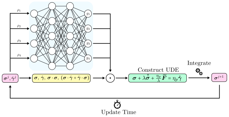
The authors establish that a Tensor-Basis Neural Network forming a Universal Differential Equation, wrapped around the upper-convected Maxwell model and trained only on small- and large-amplitude oscillatory shear data, can be deployed inside a finite-volume CFD solver and remain stable at high Deborah numbers when the tensor basis is reduced to the four terms {σ, γ̇, σ·σ, σ·γ̇ + γ̇·σ}. In this reduced formulation, the UDEs reproduce benchmark flow features—corner vortex length in 4:1 contractions and the supercritical symmetry-breaking bifurcation in cross-slot flow—with near-quantitative agreement at low De and qualitative agreement at higher De, despite the neural network not recovering t
What carries the argument
The central object is the reduced two-dimensional integrity basis for symmetric tensors, T = {σ, γ̇, σ·σ, σ·γ̇ + γ̇·σ}, used as the projection space for the TBNN output. It carries frame-invariance—any linear combination with invariant-dependent coefficients is objective—while deliberately excluding higher-order 3D tensor interactions that the authors argue are unnecessary for common constitutive models and that cause numerical instability in CFD. The UDE structure (base model plus neural correction) and the trace-based scalar invariants ρ_i as inputs complete the machinery: the network learns coefficient functions g_i(ρ) that multiply the basis tensors.
Load-bearing premise
The load-bearing premise is that the four-term two-dimensional tensor basis {σ, γ̇, σ·σ, σ·γ̇ + γ̇·σ} captures all stress–strain-rate interactions that matter in fully three-dimensional viscoelastic flows; if a real 3D flow activates higher-order tensor interactions that this basis cannot express, the learned model is structurally incomplete no matter how much data it is trained on.
What would settle it
Train the same UDE with the 4-basis formulation on the same LAOS shear data, then deploy it in a 3D flow where the third invariant tr(γ̇·γ̇·γ̇) is non-zero and significant (e.g., a 4:1 square-square contraction at De=10 or a twisted channel), and compare the stress field and stability against the ground-truth classical model. If the UDE fails well before the classical model's stability limit, the sufficiency of the 2D basis for 3D flows is falsified. Alternatively, for a real fluid, train on LAOS data, simulate a cross-slot above the measured critical Deborah number, and check whether the pred
If this is right
- Shear-only LAOS measurements on a real fluid could be used to build a constitutive model for CFD simulation of complex flows, bypassing the need to select and fit a classical model form a priori.
- The stability gain means data-driven constitutive models can be pushed to high Deborah numbers (e.g., De=20 in a planar contraction), enabling simulation of strongly elastic flows that previously were inaccessible to ML-based constitutive closures.
- The extrapolation-region diagnostic gives practitioners a way to know where a learned model is being trusted beyond its training data, suggesting that simulation results outside that envelope should be treated as qualitative only.
- Adding the first normal stress difference to the training loss is a cheap way to extend predictive fidelity to higher Deborah numbers and improve extensional-viscosity estimates, without needing extensional flow data.
Where Pith is reading between the lines
- If the 4-term basis is indeed sufficient, then any rheological behaviour that cannot be represented by this basis in 3D lies outside the scope of this modelling approach; a testable extension is to train on planar extensional data and see whether the current shear-only UDEs' shortfall in extensional hardening overshoot at high strain rates is corrected.
- The authors' observation that the TBNN rarely recovers the parsimonious ground-truth equation suggests that model identifiability is not what makes these UDEs useful; what matters is whether the learned coefficient functions produce the right flow-level observables, so validation should target benchmark observables (vortex length, bifurcation points) rather than coefficient recovery.
- The instability mechanism identified—noise in the coefficient of the quartic tensor term being amplified at inlet singularities—likely applies to other data-driven constitutive models using higher-order integrity bases, so the reduced basis may become a standard design choice for CFD-coupled learning.
- A direct extension would be to test whether the same reduced-basis UDE can extrapolate from shear training to a genuinely 3D flow with a non-trivial third invariant (e.g., a square-square contraction at higher De), since the paper's only full-3D evidence is at De=4.
Editorial analysis
A structured set of objections, weighed in public.
Referee Report
Summary. The paper presents a hybrid Tensor Basis Neural Network (TBNN) Universal Differential Equation (UDE) framework for viscoelastic constitutive modelling, integrated into an OpenFOAM/rheoTool finite-volume solver. A reduced four-tensor integrity basis — {σ, γdot, σ·σ, σ·γdot+γdot·σ} — is introduced, motivated by 2D rheometric training data and improved numerical stability. The UDEs are trained on synthetic LAOS data from Giesekus, Johnson-Segalman, sPTT/LPTT, and ePTT models, and then deployed in start-up shear/extension, 2D planar contraction, 3D square-square contraction, and planar cross-slot flows. The central claims are that the reduced basis improves stability, enables high-Deborah-number CFD simulations, and that the trained UDEs generalise beyond their shear-only training to capture extensional-flow features and elastic instabilities, with added first-normal-stress-difference information improving fidelity.
Significance. If the claims hold, the paper is a valuable contribution to hybrid ML constitutive modelling: it provides an open-source CFD implementation, a controlled bias-injection experiment isolating a numerical-stability mechanism, and an honest analysis of model identifiability and extrapolation regimes. The Giesekus and Johnson-Segalman recoveries are clean and the vortex-length agreement with Alves et al. (within 0.4%) is strong evidence of a working pipeline. The cross-slot and contraction tests, while not perfect, demonstrate that a shear-trained UDE can qualitatively capture extensional-flow and instability features. The main risk is that the central generalization claim rests on the 2D-motivated basis being sufficient for full 3D flows, an assumption tested by only a single 3D benchmark.
major comments (4)
- [§3, Eqs. (6)–(10); §6.4.2] The central claim that the reduced 2D integrity basis {σ, γdot, σ·σ, σ·γdot+γdot·σ} is sufficient for full 3D constitutive modelling is not established. The argument in §3 that 'most commonly used constitutive models' do not use the higher-order tensors of Eqs. (7)–(8) is a statement about a few benchmark models, not a completeness proof. The single 3D test in §6.4.2 is a square-square contraction at De=4 for an sPTT-trained UDE; sPTT's correction term lies entirely in the 2D subspace, so the test cannot detect the absence of the missing 3D invariants (e.g., tr(γdot^3), tr(σ·γdot^2), tr(σ^2·γdot)). Consequently, the abstract's statement that the framework 'generalise[s] beyond ... training regime' is broader than the evidence. Please either add a 3D deployment with a ground-truth model whose nonlinearity involves γdot·γdot or another excluded tensor, or restrict the claim to the tested m
- [§6.3, §6.4.1, §7] The numerical-stability advantage is convincingly demonstrated for the Giesekus-trained UDE, where the learned network degenerates to the exact Giesekus model (g3≈α, other coefficients ≈0) and the bias-injection test pinpoints the quartic term as the instability source. However, the same stability margin is not shown for the PTT/ePTT UDEs, whose coefficients are non-constant: the ePTT UDE in §6.4.1 still diverges at De=100 and no comparison to the 8/9-basis ePTT UDE is given. The conclusion that the reduced basis 'allows simulation of flows at high Deborah numbers' should be scoped to the near-exact-recovery case; for complex learned coefficients, the stability gain is plausible but quantitatively unquantified.
- [§6.1.2, §6.5, Abstract] The abstract's phrase 'data-efficient discovery of ... constitutive models' overstates the PTT results. For sPTT/ePTT, the cross-component validation loss plateaus orders of magnitude above the training loss (Fig. 7b) and the learned coefficient maps do not resemble the parsimonious ground truth (Figs. 9–11). In the cross-slot, the shear-only UDE delays the bifurcation (onset between De=0.52 and 0.54 vs ground-truth ~0.508) and the N1-trained UDE predicts a small asymmetry already at De=0.50, with centreline stress 10% high/low. 'Capturing the onset and growth of elastic instabilities' is therefore only qualitatively true. Please revise the abstract and conclusion to state that the instability is reproduced qualitatively, with quantitative accuracy dependent on training information.
- [§3, Eqs. (5)–(6)] The replacement of the identity tensor by σ·σ in the basis deserves a caveat. From the 2D Cayley–Hamilton relation, σ·σ = tr(σ)σ − det(σ)I, so an isotropic contribution c I can only be represented by a coefficient g3 = −c/det(σ) on σ·σ. This is singular when det(σ)=0, a state that can occur in general 3D flows (e.g., at stagnation points or in purely extensional kinematics with one zero principal stress). The paper argues that det(σ)=0 is 'not problematic,' but this is only true as long as no isotropic term is needed. If the goal is a general frame-invariant constitutive model, the basis should either retain I with a quiescence penalty or the limitation must be explicit.
minor comments (6)
- [Eq. (3)] Equation (3) contains corrupted control characters ('⌟⟨⟨⟪rl⟫l⟩⟩...') that must be cleaned for publication.
- [§6.5] Typo: 'the ground truth constitutive modelare almost indistinguishable' should read 'the ground-truth constitutive model is almost indistinguishable' or similar.
- [Data Availability] The statement 'available upon reasonable request' is weak for a reproducibility-focused ML paper; consider releasing trained network weights, training scripts, and the UDE model class for rheoTool.
- [§6.3] Wording: 'the basis tensor in σ⋅σ⋅γdot⋅γdot+...' should be 'the basis tensor σ⋅σ⋅γdot⋅γdot+...'.
- [§3] The quiescence penalty is described as anticipated but never implemented or tested; clarify whether it is used in the final training pipeline or only motivates the choice to exclude I.
- [§4.2] The hyperparameters κ=0.001 and w_cyc=1e-6 are fixed without sensitivity analysis; a short robustness statement would strengthen the training methodology.
Circularity Check
No significant circularity: LAOS-trained UDEs are genuinely extrapolated to contraction/cross-slot flows; Giesekus recovery is explicitly acknowledged to be by construction and is not load-bearing.
full rationale
The paper's central claim is that a TBNN-UDE trained only on oscillatory shear data generalises to unseen flow types (extension, contraction, cross-slot) when embedded in CFD. The derivation chain is not circular: the network is fitted to transient shear stress signals (Eq. 12) and optionally N1 (Eq. 13), while the evaluation targets—extensional viscosity, corner vortex lengths, and the cross-slot symmetry-breaking bifurcation—are emergent outputs of the learned constitutive model in new kinematics, not refits of the training observables. The paper is transparent that Giesekus recovery is partly by construction: it states 'the Giesekus model is a particular case in which the TBNN can effectively recover the true constitutive model' and later 'this level of model recovery is an exception rather than the rule.' Because the basis includes sigma·sigma (Eq. 6), the Giesekus target alpha*sigma·sigma coincides with a single basis coefficient (Eq. 11); the paper explicitly treats this as an expected control, not as the central evidence. The load-bearing tests are the sPTT and ePTT UDEs, for which the network does NOT recover the parsimonious ground-truth (Sec. 6.1.2) yet still produces qualitatively and semi-quantitatively correct contraction and cross-slot behaviour—a genuine extrapolation test. Validation against external benchmarks [8] and [70] (Alves et al.; Cruz et al.) provides independent support, and no derivation step relies on a self-citation chain. The restricted 2D basis in 3D is an explicitly stated modelling assumption ('this choice restricts the model class to a subset of all 3D frame invariant constitutive relations'), and the single 3D test (Sec. 6.4.2) is acknowledged as a narrow check; this is a correctness/generality limitation, not a circular reduction of the prediction to its input. No fitted parameter is renamed as a prediction, and no uniqueness theorem is imported from the authors' own prior work. Therefore no specific circular step can be exhibited.
Axiom & Free-Parameter Ledger
free parameters (4)
- TBNN weights and biases =
not reported (trained weights not shipped)
- L1 regularisation weight κ =
0.001
- Cyclic penalty weight w_cyc =
1e-6
- Hidden-layer architecture =
2 hidden layers × 32 neurons
axioms (6)
- standard math Cayley-Hamilton theorem in 2D gives a minimal basis {I, σ, γdot}.
- domain assumption Stress and strain-rate are the only tensorial flow quantities influencing stress evolution.
- domain assumption The quartic basis term σ·σ·γdot·γdot + γdot·γdot·σ·σ is not required for a valid representation.
- domain assumption A 2D-reduced basis remains adequate for fully 3D flows because common constitutive models rarely use higher-order tensor products.
- domain assumption The UCM model is an adequate base model for the UDE correction.
- standard math Neural networks are universal approximators and can represent the required correction term.
Cite this review
Pith. "Pith review of Harnessing Machine Learning for Hybrid Constitutive Modelling of Viscoelastic Fluid Flows in Computational Rheology." pith.science (2026). https://pith.science/paper/CADPEYOD
@misc{pith2026260714944,
  author       = {Pith},
  title        = {Pith review of: Harnessing Machine Learning for Hybrid Constitutive Modelling of Viscoelastic Fluid Flows in Computational Rheology},
  year         = {2026},
  howpublished = {\url{https://pith.science/paper/CADPEYOD}},
  note         = {Machine review of arXiv:2607.14944}
}
read the original abstract
Recent advances in data-driven modelling have highlighted the potential of hybrid approaches which combine Tensor Basis Neural Networks (TBNN) with Universal Differential Equations (UDE) to discover frame-invariant, non-linear viscoelastic constitutive models. These hybrid models enable the creation of digital twins for complex viscoelastic fluids, offering direct transferability to computational fluid dynamics simulations. In this work, we introduce a reduced dimensional tensor basis formulation that enhances both the physical consistency of the learned representations with respect to the training data and the numerical stability of subsequent simulations. The UDE architecture is embedded into an open-source finite volume solver in which the constitutive response is generated dynamically at runtime based on local fluid flow conditions. Training on synthetic datasets generated using a range of well established viscoelastic models in oscillatory shear flows alone, the performance of the resulting UDEs is evaluated under extrapolation to unseen conditions and flow-types. These include deploying the UDEs in viscometric extensional flows as well as 2D and 3D benchmark flows, such as the 4:1 sudden contraction and cross-slot, providing a quantitative analysis of their capabilities, limitations and failure modes. The proposed reduced-basis framework enables data-efficient discovery of frame-invariant constitutive models that generalise beyond their training regime, capturing key flow features such as the onset and growth of flow-induced elastic instabilities in strong extensional flows even though trained solely on shear data. Quantitative accuracy decreases as extrapolation increases, but incorporating first normal stress difference information further improves quantitative accuracy and extends predictive fidelity to higher Deborah numbers.
Figures


Reference graph
Works this paper leans on
-
[1]
On the formulation of rheological equations of state
Oldroyd J. G. “On the formulation of rheological equations of state”.Proceedings of the Royal Society of London. Series A. Mathematical and Physical Sciences200 (1950), pp. 523–541
1950
-
[2]
A simple constitutive equation for polymer fluids based on the concept of deformation-dependent tensorial mobility
Giesekus H. “A simple constitutive equation for polymer fluids based on the concept of deformation-dependent tensorial mobility”.Journal of Non-Newtonian Fluid Mechanics11 (1982), pp. 69–109
1982
-
[3]
A new constitutive equation derived from network theory
Phan-Thien N., Tanner R. I. “A new constitutive equation derived from network theory”.Journal of Non- Newtonian Fluid Mechanics2 (1977), pp. 353–365
1977
-
[4]
Generalized viscoelastic models: their fractional equa- tions with solutions
Schiessel H., Metzler R., Blumen A., Nonnenmacher T. “Generalized viscoelastic models: their fractional equa- tions with solutions”.Journal of physics A: Mathematical and General28 (1995), pp. 6567–6584
1995
-
[5]
Numerical simulation of non-linear elastic flows with a general collocated finite-volume method
Oliveira P. J., Pinho F. T., Pinto G. “Numerical simulation of non-linear elastic flows with a general collocated finite-volume method”.Journal of Non-Newtonian Fluid Mechanics79 (1998), pp. 1–43
1998
-
[6]
Stabilization of an open-source finite-volume solver for viscoelastic fluid flows
Pimenta F., Alves M. “Stabilization of an open-source finite-volume solver for viscoelastic fluid flows”.Journal of Non-Newtonian Fluid Mechanics239 (2017), pp. 85–104
2017
-
[7]
Popinet S.Basilisk.url:https://basilisk.fr/
-
[8]
Benchmark solutions for the flow of Oldroyd-B and PTT fluids in planar contractions
Alves M. A., Oliveira P. J., Pinho F. T. “Benchmark solutions for the flow of Oldroyd-B and PTT fluids in planar contractions”.Journal of Non-Newtonian Fluid Mechanics110 (2003), pp. 45–75
2003
-
[9]
nn-PINNs: Non-Newtonian physics-informed neural networks for complex fluid modeling
Mahmoudabadbozchelou M., Karniadakis G. E., Jamali S. “nn-PINNs: Non-Newtonian physics-informed neural networks for complex fluid modeling”.Soft Matter18 (2022), pp. 172–185
2022
-
[10]
RheologyNet: A physics-informed neural network solution to evaluate the thixotropic properties of cementitious materials
Zhang T., Wang D., Lu Y. “RheologyNet: A physics-informed neural network solution to evaluate the thixotropic properties of cementitious materials”.Cement and concrete research168 (2023), p. 107157
2023
-
[11]
ViscoelasticNet: A physics informed neural network framework for stress discovery and model selection
Thakur S., Raissi M., Ardekani A. M. “ViscoelasticNet: A physics informed neural network framework for stress discovery and model selection”.Journal of Non-Newtonian Fluid Mechanics330 (2024), p. 105265
2024
-
[12]
Data-driven selection of constitutive models via rheology- informed neural networks (RhINNs)
Saadat M., Mahmoudabadbozchelou M., Jamali S. “Data-driven selection of constitutive models via rheology- informed neural networks (RhINNs)”.Rheologica Acta61 (2022), pp. 721–732
2022
-
[13]
Data-driven constitutive model of complex fluids using recurrent neural networks
Jin H., Yoon S., Park F. C., Ahn K. H. “Data-driven constitutive model of complex fluids using recurrent neural networks”.Rheologica Acta62 (2023), pp. 569–586
2023
-
[14]
Recurrent neural networks (RNNs) learn the constitutive law of viscoelasticity
Chen G. “Recurrent neural networks (RNNs) learn the constitutive law of viscoelasticity”.Computational Me- chanics67 (2021), pp. 1009–1019
2021
-
[15]
One test to predict them all: Rheological characterization of complex fluids via artificial neural network
Mishra A. A., Ghai V., Matovic V., Arlov D., K´ ad´ ar R. “One test to predict them all: Rheological characterization of complex fluids via artificial neural network”.Engineering Applications of Artificial Intelligence139 (2025), p. 109598
2025
-
[16]
RheOFormer: A generative transformer model for simulation of complex fluids and flows
Saberi M., Farimani A. B., Jamali S. “RheOFormer: A generative transformer model for simulation of complex fluids and flows”.arXiv preprint arXiv:2510.01365(2025)
arXiv 2025
-
[17]
Rheo-SINDy: Finding a constitutive model from rheological data for complex fluids using sparse identification for nonlinear dynamics
Sato T., Miyamoto S., Kato S. “Rheo-SINDy: Finding a constitutive model from rheological data for complex fluids using sparse identification for nonlinear dynamics”.Journal of Rheology69 (2025), pp. 15–34
2025
-
[18]
Sparse regression for discovery of constitutive models from oscillatory shear mea- surements
Shanbhag S., Erlebacher G. “Sparse regression for discovery of constitutive models from oscillatory shear mea- surements”.Physics of Fluids36 (2024)
2024
-
[19]
Hammering at the entropy: a GENERIC- guided approach to learning polymeric rheological constitutive equations using PINNs
Simavilla D. N., Bonfanti A., Garc ´ ıa-Beristain I., Espa˜ nol P., Ellero M. “Hammering at the entropy: a GENERIC- guided approach to learning polymeric rheological constitutive equations using PINNs”.Journal of Fluid Me- chanics1016 (2025), A11
2025
-
[20]
Cfd-Nn Coupling for the Simulation of Complex Fluids
Darves-Blanc Q., Hippolyte A., Martin S., Macqueron C., William J., Kauric G., Abibatou N., Bonnefoy O. “Cfd-Nn Coupling for the Simulation of Complex Fluids”.Available at SSRN 4748606(2024)
2024
-
[21]
Scientific machine learning for modeling and simulating complex fluids
Lennon K. R., McKinley G. H., Swan J. W. “Scientific machine learning for modeling and simulating complex fluids”.Proceedings of the National Academy of Sciences120 (2023), e2304669120. 31
2023
-
[22]
Learning constitutive models and rheology from partial flow measurements
Sunol A. M., Roggeveen J. V., Alhashim M. G., Bae H. S., Brenner M. P. “Learning constitutive models and rheology from partial flow measurements”.arXiv preprint arXiv:2510.24673(2025)
arXiv 2025
-
[23]
Unbiased construction of constitutive relations for soft materials from experiments via rheology-informed neural networks
Mahmoudabadbozchelou M., Kamani K. M., Rogers S. A., Jamali S. “Unbiased construction of constitutive relations for soft materials from experiments via rheology-informed neural networks”.Proceedings of the National Academy of Sciences121 (2024), e2313658121
2024
-
[24]
Learning a family of rheological constitutive models using neural operators
Mangal D., Saadat M., Jamali S. “Learning a family of rheological constitutive models using neural operators”. Journal of Rheology69 (2025), pp. 55–67
2025
-
[25]
Data- driven physics-informed constitutive metamodeling of complex fluids: A multifidelity neural network (MFNN) framework
Mahmoudabadbozchelou M., Caggioni M., Shahsavari S., Hartt W. H., Karniadakis G. E., Jamali S. “Data- driven physics-informed constitutive metamodeling of complex fluids: A multifidelity neural network (MFNN) framework”.Journal of Rheology65 (2021), pp. 179–198
2021
-
[26]
Machine learning for viscoelastic constitutive model identification and parameterisation using large amplitude oscillatory shear
John T. P., Mowbray M., Alalwyat A., Vousvoukis M., Martin P., Kowalski A., Fonte C. P. “Machine learning for viscoelastic constitutive model identification and parameterisation using large amplitude oscillatory shear”. Chemical Engineering Science294 (2024), p. 120075
2024
-
[27]
Digital rheometer twins: Learning the hidden rheology of complex fluids through rheology-informed graph neural networks
Mahmoudabadbozchelou M., Kamani K. M., Rogers S. A., Jamali S. “Digital rheometer twins: Learning the hidden rheology of complex fluids through rheology-informed graph neural networks”.Proceedings of the National Academy of Sciences119 (2022), e2202234119
2022
-
[28]
Pinnsformer: A transformer-based framework for physics-informed neural networks
Zhao Z., Ding X., Prakash B. A. “Pinnsformer: A transformer-based framework for physics-informed neural networks”.arXiv preprint arXiv:2307.11833(2023)
Pith/arXiv arXiv 2023
-
[29]
Attention is all you need
Vaswani A., Shazeer N., Parmar N., Uszkoreit J., Jones L., Gomez A. N., Kaiser L., Polosukhin I. “Attention is all you need”.Advances in neural information processing systems30 (2017)
2017
-
[30]
Fourier neural operator for parametric partial differential equations
Li Z., Kovachki N., Azizzadenesheli K., Liu B., Bhattacharya K., Stuart A., Anandkumar A. “Fourier neural operator for parametric partial differential equations”.arXiv preprint arXiv:2010.08895(2020)
Pith/arXiv arXiv 2010
-
[31]
A composite neural network that learns from multi-fidelity data: Application to function approximation and inverse PDE problems
Meng X., Karniadakis G. E. “A composite neural network that learns from multi-fidelity data: Application to function approximation and inverse PDE problems”.Journal of Computational Physics401 (2020), p. 109020
2020
-
[32]
Multiscale simulations for viscoelastic fluids with approximate constitutive models derived by a sparse identification method
Sato T., Miyamoto S. “Multiscale simulations for viscoelastic fluids with approximate constitutive models derived by a sparse identification method”.Rheologica Acta(2025), pp. 1–17
2025
-
[33]
A survey on the application of machine learning in turbulent flow simulations
Majchrzak M., Marciniak-Lukasiak K., Lukasiak P. “A survey on the application of machine learning in turbulent flow simulations”.Energies16 (2023), p. 1755
2023
-
[34]
Reynolds averaged turbulence modelling using deep neural networks with embedded invariance
Ling J., Kurzawski A., Templeton J. “Reynolds averaged turbulence modelling using deep neural networks with embedded invariance”.Journal of Fluid Mechanics807 (2016), pp. 155–166
2016
-
[35]
Finding the underlying viscoelastic constitutive equation via universal differential equations and differentiable physics
Rodrigues E. C., Thompson R. L., Oliveira D. A., Ausas R. F. “Finding the underlying viscoelastic constitutive equation via universal differential equations and differentiable physics”.Engineering Applications of Artificial Intelligence160 (2025), p. 111788
2025
-
[36]
Discovering governing equations from data by sparse identification of nonlinear dynamical systems
Brunton S. L., Proctor J. L., Kutz J. N. “Discovering governing equations from data by sparse identification of nonlinear dynamical systems”.Proceedings of the national academy of sciences113 (2016), pp. 3932–3937
2016
-
[37]
On the high Weissenberg number problem
Keunings R. “On the high Weissenberg number problem”.Journal of Non-Newtonian Fluid Mechanics20 (1986), pp. 209–226
1986
-
[38]
The log-conformation tensor approach in the finite-volume method framework
Afonso A., Oliveira P. J., Pinho F. T., Alves M. A. “The log-conformation tensor approach in the finite-volume method framework”.Journal of Non-Newtonian Fluid Mechanics157 (2009), pp. 55–65
2009
-
[39]
Numerical methods for viscoelastic fluid flows
Alves M. A., Oliveira P. J., Pinho F. T. “Numerical methods for viscoelastic fluid flows”.Annual Review of Fluid Mechanics53 (2021), pp. 509–541
2021
-
[40]
Universal differential equations for scientific machine learning
Rackauckas C., Ma Y., Martensen J., Warner C., Zubov K., Supekar R., Skinner D., Ramadhan A., Edelman A. “Universal differential equations for scientific machine learning”.arXiv preprint arXiv:2001.04385(2020)
Pith/arXiv arXiv 2001
-
[41]
Neural ordinary differential equations
Chen R. T. Q., Rubanova Y., Bettencourt J., Duvenaud D. K. “Neural ordinary differential equations”.Advances in neural information processing systems31 (2018)
2018
-
[42]
Multilayer feedforward networks are universal approximators
Hornik K., Stinchcombe M., White H. “Multilayer feedforward networks are universal approximators”.Neural networks2 (1989), pp. 359–366
1989
-
[43]
The theory of matrix polynomials and its application to the mechanics of isotropic continua
Spencer A. J. M., Rivlin R. S. “The theory of matrix polynomials and its application to the mechanics of isotropic continua”.Archive for rational mechanics and analysis2 (1958), pp. 309–336
1958
-
[44]
On isotropic functions of symmetric tensors, skew-symmetric tensors and vectors
Smith G. “On isotropic functions of symmetric tensors, skew-symmetric tensors and vectors”.International journal of engineering science9 (1971), pp. 899–916
1971
-
[45]
Clarifying the representation of isotropic symmetric tensor-valued functions of two symmetric tensors
Kamrin K., Govindjee S. “Clarifying the representation of isotropic symmetric tensor-valued functions of two symmetric tensors”.Mathematics and Mechanics of Solids31 (2026), pp. 172–182. 32
2026
-
[46]
Enforcing Dirichlet boundary conditions in physics-informed neural networks and variational physics-informed neural networks
Berrone S., Canuto C., Pintore M., Sukumar N. “Enforcing Dirichlet boundary conditions in physics-informed neural networks and variational physics-informed neural networks”.Heliyon9 (2023)
2023
-
[47]
F.The theory of Polymer Dynamics
Doi M., Edwards S. F.The theory of Polymer Dynamics. 1986
1986
-
[48]
Pytorch: An imperative style, high-performance deep learning library
Paszke A., Gross S., Massa F., Lerer A., Bradbury J., Chanan G., Killeen T., Lin Z., Gimelshein N., Antiga L., et al. “Pytorch: An imperative style, high-performance deep learning library”.Advances in neural information processing systems32 (2019)
2019
-
[49]
Compiling machine learning programs via high-level tracing
Frostig R., Johnson M. J., Leary C. “Compiling machine learning programs via high-level tracing”.SysML conference 2018. 2019
2018
-
[50]
Jakob W.pybind11 Documentation. 2024
2024
-
[51]
Rodriguez S., Cardiff P. “A general approach for running Python codes in OpenFOAM using an embedded Pybind11 Python interpreter”.arXiv preprint arXiv:2203.16394(2022)
arXiv 2022
-
[52]
Understanding the difficulty of training deep feedforward neural networks
Glorot X., Bengio Y. “Understanding the difficulty of training deep feedforward neural networks”.Proceedings of the thirteenth international conference on artificial intelligence and statistics. JMLR Workshop and Conference Proceedings. 2010, pp. 249–256
2010
-
[53]
Batch normalization: Accelerating deep network training by reducing internal covariate shift
Ioffe S., Szegedy C. “Batch normalization: Accelerating deep network training by reducing internal covariate shift”.International conference on machine learning. pmlr. 2015, pp. 448–456
2015
-
[54]
A review of nonlinear oscillatory shear tests: Analysis and application of large amplitude oscillatory shear (LAOS)
Hyun K., Wilhelm M., Klein C. O., Cho K. S., Nam J. G., Ahn K. H., Lee S. J., Ewoldt R. H., McKinley G. H. “A review of nonlinear oscillatory shear tests: Analysis and application of large amplitude oscillatory shear (LAOS)”.Progress in polymer science36 (2011), pp. 1697–1753
2011
-
[55]
Self-consistent Fourier–Tschebyshev rep- resentations of the first normal stress difference in large amplitude oscillatory shear
King N., Pashkovski E., Patterson R., Rockwell P., McKinley G. H. “Self-consistent Fourier–Tschebyshev rep- resentations of the first normal stress difference in large amplitude oscillatory shear”.Journal of Rheology70 (2026), pp. 307–327
2026
-
[56]
Tuor A., Drgona J., Vrabie D.Constrained neural ordinary differential equations with stability guarantees. 2020
2020
-
[57]
Thummerer T., Mikelsons L.Eigen-informed neural ordinary differential equations: Incorporating knowledge of system properties. 2025
2025
-
[58]
Adam: A method for stochastic optimization
Kingma D. P. “Adam: A method for stochastic optimization”.arXiv preprint arXiv:1412.6980(2014)
Pith/arXiv arXiv 2014
-
[59]
On the limited memory BFGS method for large scale optimization
Liu D. C., Nocedal J. “On the limited memory BFGS method for large scale optimization”.Mathematical programming45 (1989), pp. 503–528
1989
-
[60]
An overview of overfitting and its solutions
Ying X. “An overview of overfitting and its solutions”.Journal of physics: Conference series. Vol. 1168. IOP Publishing. 2019, p. 022022
2019
-
[61]
A nonlinear network viscoelastic model
Phan-Thien N. “A nonlinear network viscoelastic model”.Journal of Rheology22 (1978), pp. 259–283
1978
-
[62]
Working group on numerical techniques
Hassager O. “Working group on numerical techniques”.J. of Non-Newtonian Fluid Mech.29 (1988), pp. 2–5
1988
-
[63]
Dynamics of high-Deborah-number entry flows: a numerical study
Afonso A. M., Oliveira P. J., Pinho F. T., Alves M. A. “Dynamics of high-Deborah-number entry flows: a numerical study”.Journal of Fluid Mechanics677 (2011), pp. 272–304
2011
-
[64]
Numerical simulation of the planar contraction flow of a Giesekus fluid
Choi H. C., Song J. H., Yoo J. Y. “Numerical simulation of the planar contraction flow of a Giesekus fluid”. Journal of Non-Newtonian Fluid Mechanics29 (1988), pp. 347–379
1988
-
[65]
Effect of the contraction ratio upon viscoelastic fluid flow in three-dimensional square–square contractions
Sousa P. C., Coelho P. M., Oliveira M. S. N., Alves M. A. “Effect of the contraction ratio upon viscoelastic fluid flow in three-dimensional square–square contractions”.Chemical Engineering Science66 (2011), pp. 998–1009
2011
-
[66]
Extrapolation limitations of multilayer feedforward neural networks
Haley P. J., Soloway D. “Extrapolation limitations of multilayer feedforward neural networks”.[Proceedings 1992] IJCNN international joint conference on neural networks. Vol. 4. IEEE. 1992, pp. 25–30
1992
-
[67]
Large amplitude oscilla- tory extension (LAOE) of dilute polymer solutions
Recktenwald S. M., John T. P., Shen A. Q., Poole R. J., Fonte C. P., Haward S. J. “Large amplitude oscilla- tory extension (LAOE) of dilute polymer solutions”.Journal of Non-Newtonian Fluid Mechanics342 (2025), p. 105421
2025
-
[68]
Optimized cross-slot flow geometry for microfluidic extensional rheometry
Haward S. J., Oliveira M. S. N., Alves M. A., McKinley G. H. “Optimized cross-slot flow geometry for microfluidic extensional rheometry”.Physical Review Letters109 (2012), p. 128301
2012
-
[69]
Purely elastic flow asymmetries
Poole R. J., Alves M. A., Oliveira P. J. “Purely elastic flow asymmetries”.Physical review letters99 (2007), p. 164503
2007
-
[70]
A new viscoelastic benchmark flow: Stationary bifurcation in a cross-slot
Cruz F. A., Poole R. J., Afonso A. M., Pinho F. T., Oliveira P. J., Alves M. A. “A new viscoelastic benchmark flow: Stationary bifurcation in a cross-slot”.Journal of Non-Newtonian Fluid Mechanics214 (2014), pp. 57–68
2014
-
[71]
On extensibility effects in the cross-slot flow bifurcation
Rocha G. N., Poole R. J., Alves M. A., Oliveira P. J. “On extensibility effects in the cross-slot flow bifurcation”. Journal of Non-Newtonian Fluid Mechanics156 (2009), pp. 58–69. 33
2009
discussion (0)
Sign in with ORCID, Apple, or X to comment. Anyone can read and Pith papers without signing in.