REVIEW 2 major objections 2 minor 1 cited by
Deep learning applied to computational mechanics: A comprehensive review, state of the art, and the classics
T0 review · 2 major / 2 minor · reviewed 2026-05-24 · grok-4.3
Pith's one-line read Deep learning methods, both hybrid and pure, are reviewed for use in solid and fluid mechanics simulations.
desk verdict This review builds DL concepts from basics for mechanics readers and flags some AI misconceptions, but its value as state-of-the-art coverage rests on whether the citations are representative. read the letter →
The pith
A machine-rendered reading of the paper's core claim, the machinery that carries it, and where it could break.
The reading
What carries the argument
Hybrid methods that augment traditional PDE discretizations with ML and pure ML methods such as physics-informed neural networks, with LSTM for constitutive modeling and model reduction and attention for discontinuities.
What would settle it
Discovery of a substantial number of peer-reviewed works on deep learning for finite-element or continuum mechanics problems that are omitted from the review would indicate the coverage is incomplete.
Extended reading notes
Core claim
The paper claims that recent deep learning developments relevant to computational mechanics can be organized into hybrid methods, which use LSTM networks to model nonlinear constitutive relations or reduce model order and convolutional networks to accelerate traditional integrators, and pure ML methods represented by physics-informed neural networks that may incorporate attention to handle discontinuous solutions; it further reviews LSTM and attention architectures along with stochastic optimizers and kernel machines to sufficient depth for advanced follow-on work.
Load-bearing premise
The chosen papers and methods accurately represent the current state of the art without significant selection bias or major omissions.
Editorial extensions
If this is right
- Hybrid LSTM-based methods can capture complex nonlinear material behavior within existing finite-element frameworks.
- Model-order reduction via LSTM can make turbulence simulations more efficient.
- Convolutional networks can speed up specific steps inside conventional time-integration schemes.
- PINNs, possibly augmented with attention, can solve nonlinear PDEs directly without traditional discretization.
- Kernel machines including Gaussian processes provide a foundation for understanding infinite-width shallow networks.
Reading between the lines
- The review structure could serve as a template for similar surveys in related fields such as structural optimization or multiphysics coupling.
- Explicit discussion of limitations in the classics may encourage more careful citation practices when referencing early AI work in engineering contexts.
- The beam-positioning example suggests that the reviewed techniques are already close to practical control applications in deformable-body dynamics.
Editorial analysis
A structured set of objections, weighed in public.
Referee Report
Summary. The manuscript is a review paper surveying recent deep learning applications to computational mechanics. It covers hybrid methods that combine traditional PDE discretizations with LSTM (for constitutive modeling and model-order reduction) and CNN (for simulation acceleration), pure ML approaches such as PINNs with attention mechanisms for discontinuous solutions, reviews of LSTM/attention architectures, modern optimizers, and kernel machines (including Gaussian processes and infinite-width networks), plus discussion of AI history, limitations, and misconceptions. An example application to positioning/pointing control of a large-deformable beam is included. The target audience is computational-mechanics experts new to DL, with concepts built from the basics.
Significance. If the literature selection is representative and the coverage balanced, the review would provide a useful on-ramp for mechanics researchers entering DL, explicitly contrasting hybrid and pure-ML strategies and correcting common misconceptions about the classics. The inclusion of both modern architectures and kernel-machine background for advanced readers adds pedagogical value.
major comments (2)
- [Abstract] Abstract and opening sections: the central claim that the paper reviews 'many recent developments ... in detail' and supplies the 'state of the art' rests on the assumption of unbiased, comprehensive paper selection up to the 2022 cutoff. No explicit selection methodology, inclusion/exclusion criteria, or discussion of potential gaps (e.g., key LSTM turbulence papers or additional PINN variants) is provided, making it impossible to verify representativeness.
- [Introduction (implied by abstract)] The positioning statement that the review brings 'first-time learners quickly to the forefront of research' is load-bearing for the intended contribution, yet the manuscript does not compare its scope or depth against existing surveys in the same area, leaving the incremental value of this particular synthesis unclear.
minor comments (2)
- [Abstract] The three motivating AI breakthroughs cited in the abstract are not enumerated explicitly; listing them would strengthen the opening motivation.
- Ensure that every cited work is dated no later than the stated 2022 cutoff and that references to the 'classics' are accompanied by the specific misstatements being corrected.
Simulated Author's Rebuttal
We thank the referee for the constructive comments. We address each major comment below, agreeing that additional clarifications on scope and comparisons to prior surveys will strengthen the manuscript.
read point-by-point responses
-
Referee: [Abstract] Abstract and opening sections: the central claim that the paper reviews 'many recent developments ... in detail' and supplies the 'state of the art' rests on the assumption of unbiased, comprehensive paper selection up to the 2022 cutoff. No explicit selection methodology, inclusion/exclusion criteria, or discussion of potential gaps (e.g., key LSTM turbulence papers or additional PINN variants) is provided, making it impossible to verify representativeness.
Authors: We agree that an explicit discussion of literature selection would improve transparency. Although the review was compiled based on relevance to computational mechanics applications up to the 2022 cutoff, we will add a new paragraph in the Introduction describing the general search approach, inclusion focus on solid/fluid mechanics and finite-element contexts, and explicit acknowledgment of potential gaps (e.g., certain turbulence LSTM works or post-cutoff PINN variants). revision: yes
-
Referee: [Introduction (implied by abstract)] The positioning statement that the review brings 'first-time learners quickly to the forefront of research' is load-bearing for the intended contribution, yet the manuscript does not compare its scope or depth against existing surveys in the same area, leaving the incremental value of this particular synthesis unclear.
Authors: The manuscript's distinctive elements include the joint treatment of hybrid LSTM/CNN methods with pure PINN approaches, coverage of kernel machines and infinite-width networks, and discussion of AI history with corrections to common misconceptions. We nevertheless recognize the benefit of explicit positioning. We will revise the Introduction to include a concise comparison with related surveys (e.g., those focused primarily on PINNs or data-driven constitutive modeling) and to articulate the incremental synthesis provided here. revision: yes
Circularity Check
No circularity: review draws from external citations without internal derivations
full rationale
This is a literature review paper with no original mathematical derivations, predictions, or fitted models presented as results. The central content consists of summaries of external cited works on DL methods for mechanics (LSTM, PINN, etc.), built from basics for the reader. No steps match the enumerated circularity patterns, as there are no equations reducing to inputs by construction, no fitted parameters renamed as predictions, and no load-bearing self-citations that justify a uniqueness theorem or ansatz. The paper is self-contained as a survey against external benchmarks.
Assumptions & free parameters
Cite this review
Pith. "Pith review of Deep learning applied to computational mechanics: A comprehensive review, state of the art, and the classics." pith.science (2026). https://pith.science/paper/CAVQMFLS
@misc{pith2026221208989,
  author       = {Pith},
  title        = {Pith review of: Deep learning applied to computational mechanics: A comprehensive review, state of the art, and the classics},
  year         = {2026},
  howpublished = {\url{https://pith.science/paper/CAVQMFLS}},
  note         = {Machine review of arXiv:2212.08989}
}
read the original abstract
Three recent breakthroughs due to AI in arts and science serve as motivation: An award winning digital image, protein folding, fast matrix multiplication. Many recent developments in artificial neural networks, particularly deep learning (DL), applied and relevant to computational mechanics (solid, fluids, finite-element technology) are reviewed in detail. Both hybrid and pure machine learning (ML) methods are discussed. Hybrid methods combine traditional PDE discretizations with ML methods either (1) to help model complex nonlinear constitutive relations, (2) to nonlinearly reduce the model order for efficient simulation (turbulence), or (3) to accelerate the simulation by predicting certain components in the traditional integration methods. Here, methods (1) and (2) relied on Long-Short-Term Memory (LSTM) architecture, with method (3) relying on convolutional neural networks. Pure ML methods to solve (nonlinear) PDEs are represented by Physics-Informed Neural network (PINN) methods, which could be combined with attention mechanism to address discontinuous solutions. Both LSTM and attention architectures, together with modern and generalized classic optimizers to include stochasticity for DL networks, are extensively reviewed. Kernel machines, including Gaussian processes, are provided to sufficient depth for more advanced works such as shallow networks with infinite width. Not only addressing experts, readers are assumed familiar with computational mechanics, but not with DL, whose concepts and applications are built up from the basics, aiming at bringing first-time learners quickly to the forefront of research. History and limitations of AI are recounted and discussed, with particular attention at pointing out misstatements or misconceptions of the classics, even in well-known references. Positioning and pointing control of a large-deformable beam is given as an example.
Figures


Figures from the paper (159 more)











Forward citations
Cited by 1 Pith paper
-
SLIDE: A machine-learning based method for forced dynamic response estimation of multibody systems
SLIDE is a deep learning estimator that truncates initial effects via complex eigenvalues of linearized equations to predict output sequences of damped multibody systems, reporting speedups up to several million times.
Reference graph
Works this paper leans on
-
[2]
Rosenblatt, F. (1962). Principles of neurodynamics: Perceptrons and the theory of brain mechanisms. Spartan Books. 2, 11, 46, 55, 210, 212, 213, 214, 215, 271
work page 1962
-
[3]
Polyak, B. (1964). Some methods of speeding up the convergence of iteration methods . USSR Com- putational Mathematics and Mathematical Physics, 4(5), 1–17. DOI 10.1016/0041-5553(64)90137-5. 2, 10, 11, 85, 89, 90, 91
-
[4]
Roose, K. (2022). An A.I.-Generated Picture Won an Art Prize. Artists Aren’t Happy.New York Times, (Sep 2). Original website. 6, 7
work page 2022
-
[5]
Jumper, J., Evans, R., Pritzel, A., Green, T., Figurnov, M., et al. (2021). Highly accurate protein structure prediction with AlphaFold. Nature, 596(7873), 583–589. 7
work page 2021
-
[6]
J., Guez, A., Sifre, L., et al
Silver, D., Huang, A., Maddison, C. J., Guez, A., Sifre, L., et al. (2016). Mastering the game of Go with deep neural networks and tree search. Nature, 529(7587), 484+. Original website. 7, 12, 13
work page 2016
-
[7]
How Google’s AlphaGo Beat a Go World Champion
Moyer, C. How Google’s AlphaGo Beat a Go World Champion. 2016 Mar 28, Original website. 7
work page 2016
-
[8]
Edwards, B. (2022). DeepMind breaks 50-year math record using AI; new record falls a week later. Ars Technica, (Oct 13). Original website, Internet archive. 7
work page 2022
-
[9]
Vu-Quoc, L., Humer, A. (2022). Deep learning applied to computational mechanics: A comprehensive review, state of the art, and the classics. arXiv:2212.08989. 8
work page Pith review arXiv 2022
Show all 286 references
-
[10]
Roose, K. (2023). Bing (Yes, Bing) Just Made Search Interesting Again. New York Times, (Feb 8). Original website. 8
2023
-
[11]
Knight, W. (2023). Meet Bard, Google’s Answer to ChatGPT. WIRED, (Feb 6). Original website. 8
2023
-
[12]
Schmidhuber, J. (2015). Deep learning in neural networks: An overview. Neural Networks, 61, 87–
2015
-
[13]
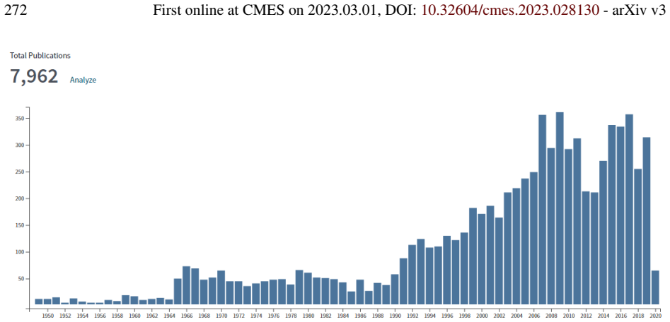
8, 36, 38, 52, 223, 224, 225, 272
-
[14]
LeCun, Y ., Bengio, Y ., Hinton, G. (2015). Deep learning.Nature, 521(7553), 436–444. 8, 12, 14, 38, 52, 53, 54, 129, 131
2015
-
[15]
Khan, S., Yairi, T. (2018). A review on the application of deep learning in system health management. Mechanical Systems and Signal Processing, 107, 241–265. 8
2018
-
[16]
Sanchez-Lengeling, B., Aspuru-Guzik, A. (2018). Inverse molecular design using machine learning: Generative models for matter engineering. Science, 361(6400, SI), 360–365. 8
2018
-
[17]
S., Beaulieu-Jones, B
Ching, T., Himmelstein, D. S., Beaulieu-Jones, B. K., Kalinin, A. A., Do, B. T., et al. (2018). Opportu- nities and obstacles for deep learning in biology and medicine. Journal of the Royal Society Interface, 15(141). 8
2018
-
[18]
A., Nyhan, M
Quinn, J. A., Nyhan, M. M., Navarro, C., Coluccia, D., Bromley, L., et al. (2018). Humanitarian applications of machine learning with remote-sensing data: review and case study in refugee settlement mapping. Philosophical Transactions of the Royal Society A-Mathematical Physic...
2018
-
[19]
F., Higham, D
Higham, C. F., Higham, D. J. (2019). Deep learning: An introduction for applied mathematicians. SIAM Review, 61(4), 860–891. 8
2019
-
[20]
Dayan, P., Abbott, L. (2001). Theoretical Neuroscience: Computational and Mathematical Modeling of Neural Systems. MIT Press. 8, 9, 11, 30, 31, 38, 39, 40, 41, 43, 212, 215, 216, 217, 219
2001
-
[21]
Sze, V ., Chen, Y .-H., Yang, T.-J., Emer, J. S. (2017). Efficient Processing of Deep Neural Networks: A Tutorial and Survey. Proceedings of the IEEE, 105(12), 2295–2329. 8, 17, 32, 38, 209
2017
-
[22]
Nielsen, M. (2015). Neural Networks and Deep Learning . Determination Press. Original website. Internet archive. 8, 32, 38, 66, 67, 209, 210, 213
2015
-
[23]
Rumelhart, D., Hinton, G., Williams, R. (1986). Learning representations by back-propagating errors. Nature, 323(6088), 533–536. 8, 90, 215, 223, 224, 225, 271
1986
-
[24]
Ghaboussi, J., Garrett, J., Wu, X. (1991). Knowledge-based modeling of material behavior with neural networks. Journal of Engineering Mechanics-ASCE, 117(1), 132–153. 8, 9, 26, 32, 173, 209, 272
1991
-
[26]
Wang, K., Sun, W. C. (2018). A multiscale multi-permeability poroplasticity model linked by recursive homogenizations and deep learning. Computer Methods in Applied Mechanics and Engineering, 334, 337–380. 8, 9, 11, 22, 24, 25, 26, 27, 28, 172, 173, 174, 175, 176, 177, 178, 17...
2018
-
[27]
Mohan, A., Gaitonde, D. (2018). A deep learning based approach to reduced order modeling for turbulent flow control using LSTM neural networks. arXiv:1804.09269 [physics.comp-ph]. Apr 24. 8, 9, 11, 28, 29, 30, 184, 185, 186, 187, 188, 189, 190, 191, 192
2018 arXiv
-
[28]
Zaman, M., Zhu, J. (1998). A neural network model for a cohesionless soilIn AttohOkine, NO. Arti- ficial Intelligence and Mathematical Methods in Pavement and Geomechanical Systems. International Workshop on Artificial Intelligence and Mathematical Methods in Pavement and Geom...
1998
-
[29]
Su, H., Fan, L., Schlup, J. (1998). Monitoring the process of curing of epoxy/graphite fiber composites with a recurrent neural network as a soft sensor. Engineering Applications of Artificial Intelligence , 11(2), 293–306. 9
1998
-
[30]
Li, C., Huang, T. (1999). Automatic structure and parameter training methods for modeling of me- chanical systems by recurrent neural networks. Applied Mathematical Modelling , 23(12), 933–944. 9
1999
-
[31]
Waszczyszyn, Z. (2000). Neural networks in structural engineering: Some recent results and prospects for applicationsIn Topping, BHV. Computational Mechanics for the Twenty-First Century. 5th Inter- national Conference on Computational Structures Technology/2nd International C...
2000
-
[32]
Vaswani, A., Shazeer, N., Parmar, N., Uszkoreit, J., Jones, L., et al. (2017). Attention Is All You Need. CoRR, abs/1706.03762v5. arXiv:1706.03762v5. See Footnote 337. 9, 11, 135, 138, 139, 140, 141, 142, 143, 248
2017 arXiv
-
[33]
Hahnloser, R., Sarpeshkar, R., Mahowald, M., Douglas, R., Seung, S. (2000). Digital selection and analogue amplification coexist in a cortex-inspired silicon circuit (vol 405, pg 947, 2000). Nature, 408(6815), 1012–U24. 9, 39, 219, 221, 222
2000
-
[34]
Jarrett, K., Kavukcuoglu, K., Ranzato, M., LeCun, Y . (2009). What is the Best Multi-Stage Architec- ture for Object Recognition?In 2009 IEEE 12th International Conference on Computer Vision (ICCV). IEEE International Conference on Computer Vision. IEEE; IEEE Comp Soc. 12th IE...
2009
-
[35]
Nair, V ., Hinton, G. (2010). Rectified linear units improve restricted boltzmann machines.Proceedings of the 27th International Conference on Machine Learning, Haifa, Israel. 9, 39
2010
-
[36]
Little, W. (1974). The existence of persistent states in the brain. Mathematical Biosciences, 19, 101–
1974
-
[37]
In Cabrera, B and Gutfreund, H and Kresin, V (eds), From High-Temperature Superconductivity to Microminiature Refrigeration, William Little Symposium on From High-Temperature Supercon- ductivity to Microminiature Refrigeration, Stanford Univ, Stanford, CA, Sep 30, 1995.336. 9, 220
1995
-
[38]
Ramachandran, P., Barret, Z., Le, Q. (2017). Searching for Activation Functions. CoRR (Computing Research Repository), abs/1710.05941v2. arXiv:1710.05941v2. See Footnote 337. 9, 52, 219, 221, 222, 223
2017 arXiv
-
[40]
Oishi, A., Yagawa, G. (2017). Computational mechanics enhanced by deep learning. Computer Meth- ods in Applied Mechanics and Engineering, 327, 327–351. 9, 11, 18, 19, 20, 21, 32, 46, 53, 60, 163, 164, 165, 166, 167, 168, 169, 170, 171, 172, 209
2017
-
[41]
Zienkiewicz, O., Taylor, R., Zhu, J. (2013). The Finite Element Method: Its Basis and Fundamentals. Oxford: Butterworth-Heineman. 7th edition. 9, 35, 163, 164
2013
-
[42]
Barlow, J. (1976). Optimal stress locations in finite-element models. International Journal for Numer- ical Methods in Engineering, 10(2), 243–251. 9
1976
-
[43]
Barlow, J. (1977). Optimal stress locations in finite-element models - reply. International Journal for Numerical Methods in Engineering, 11(3), 604. 9
1977
-
[44]
Theory Guide
Abaqus 6.14. Theory Guide. Simulia Systems, Dassault Systèmes. Subsection 3.2.4 Solid isoparamet- ric quadrilaterals and hexahedra. (Website, go to Section Reference, Abaqus Theory Guide, Section 3 Elements, Section 3.2 Continuum elements, then Section 3.2.4.). 9
-
[45]
Ghaboussi, J., Garrett, J., Wu, X. (1990). Material Modeling with Neural NetworksIn Pande, GN and Middleton, J. Numerical Methods in Engineering : Theory and Applications, Vol 2. 3rd International Conf on Numerical Methods in Engineering : Theory and Applications ( NUMETA 90 )...
1990
-
[46]
Chen, C. (1989). Applying and validating neural network technology for nondestructive evaluation of materialsIn 1989 IEEE International Conference on Systems, Man, and Cybernetics, Vols 1-3: Con- ference Proceedings. 1989 IEEE International Conf on Systems, Man, and Cybernetic...
1989
-
[47]
Sayeh, M., Viswanathan, R., Dhali, S. (1990). Neural networks for assessment of impact and stress relief on composite-materialsIn Genisio, M. Sixth Annual Conference on Materials Technology: Com- posite Technology. 6th Annual Conf on Materials Technology : Composite Technology...
1990
-
[48]
Chen, C., Leclair, S. (1991). A probability neural network (pnn) estimator for improved reliability of noisy sensor data. Journal of Reinforced Plastics and Composites, 10(4), 379–390. 9
1991
-
[49]
Kim, Y ., Choi, Y ., Widemann, D., Zohdi, T. (2020). A fast and accurate physics-informed neural network reduced order model with shallow masked autoencoderer. ( Sep 28). Version 2, 2020.09.28: arXiv:2009.11990v2, 2009.11990. 9, 10, 11, 193, 194, 195, 196, 197, 198, 199, 200, ...
2020
-
[50]
Kim, Y ., Choi, Y ., Widemann, D., Zohdi, T. (2020). Efficient nonlinear manifold reduced order model. (Nov 13). arXiv:2011.07727, 2011.07727. 9, 10, 11, 193
2020
-
[51]
Robbins, H., Monro, S. (1951b). Stochastic approximation. Annals of Mathematical Statistics, 22(2),
-
[52]
Nesterov, I. (1983). A method of the solution of the convex-programming problem with a speed of convergence O(1/k2). Doklady Akademii Nauk SSSR, 269(3), 543–547. In Russian. 10, 89, 91
1983
-
[53]
Nesterov, Y . (2018). Lecture on Convex Optimization. 2nd edition. Switzerland: Springer Nature. 10, 89, 91
2018
-
[54]
Duchi, J., Hazan, E., Singer, Y . (2011). Adaptive Subgradient Methods for Online Learning and Stochastic Optimization. Journal of Machine Learning Research, 12, 2121–2159. 10, 105
2011
-
[55]
Tieleman, T., Hinton, G. (2012). Lecture 6e, rmsprop: Divide the gradient by a running average of its recent magnitude. Youtube video, time 5:54. Lecture notes, p.29: Original website, Internet archive. 10, 108
2012
-
[56]
Zeiler, M. D. (2012). ADADELTA: An adaptive learning rate method. ( Dec 22). arXiv:1212.5701. 10, 106, 108, 109
2012 arXiv
-
[58]
Loshchilov, I., Hutter, F. (2019). Decoupled weight decay regularization. (Jan 4). arXiv:1711.05101v3. OpenReview. 10, 85, 87, 92, 93, 99, 106, 109, 115, 116, 117, 123
2019 arXiv
-
[59]
Bahdanau, D., Cho, K., Bengio, Y . (2015). Neural machine translation by jointly learning to align and translate. CoRR, abs/1409.0473. arXiv:1409.0473. 11, 135, 136, 137, 138
2015 arXiv
-
[60]
Furshpan, E., Potter, D. (1957). Mechanism of nerve-impulse transmission at a crayfish synapse. Nature, 180(4581), 342–343. 11, 222
1957
-
[61]
Furshpan, E., Potter, D. (1959b). Slow post-synaptic potentials recorded from the giant motor fibre of the crayfish. Journal of Physiology-London, 145(2), 326–335. 11, 222
-
[62]
Gershgorn, D. (2017). The data that transformed AI research—and possibly the world. Quartz, (Jul 26). Original website. Internet archive (blurry images). 11, 13
2017
-
[63]
He, K., Zhang, X., Ren, S., Sun, J. (2015). Delving Deep into Rectifiers: Surpassing Human-Level Performance on ImageNet Classification. CoRR, abs/1502.01852. arXiv:1502.01852, 1502.01852. 12, 40, 70, 206, 220
2015 arXiv
-
[64]
Russakovsky, O., Deng, J., Su, H., Krause, J., Satheesh, S., et al. (2015). ImageNet Large Scale Visual Recognition Challenge. International Journal of Computer Vision, 115(3), 211–252. 12, 13
2015
-
[65]
Park, E., Liu, W., Russakovsky, O., Deng, J., Li, F., et al. (2017). ImageNet Large scale visual recogni- tion challenge (ILSVRC) 2017, Overview. ILSVRC 2017, (Jul 26). Original website Internet archive. 12, 13
2017
-
[66]
Science’s 2021 Breakthrough: AI-powered Protein Prediction
Beckwith, W. Science’s 2021 Breakthrough: AI-powered Protein Prediction. 2022 Dec 17, Original website. 11, 12
2021
-
[67]
DeepMind, 2022 Jul 28, Original website, Internet archive
AlphaFold reveals the structure of the protein universe. DeepMind, 2022 Jul 28, Original website, Internet archive. 12
2022
-
[68]
DeepMind’s AI predicts structures for a vast trove of proteins
Callaway, E. DeepMind’s AI predicts structures for a vast trove of proteins. 2021 Jul 21, Original website. 12
2021
-
[69]
The Guardian view on the future of AI: Great power, great irresponsibility
Editorial (2019). The Guardian view on the future of AI: Great power, great irresponsibility. The Guardian, (Jan 01). Original website. Internet archive. 12, 236, 237
2019
-
[70]
Silver, D., Hubert, T., Schrittwieser, J., Antonoglou, I., Lai, M., et al. (2018). A general reinforcement learning algorithm that masters chess, shogi, and Go through self-play.Science, 362(6419), 1140+. 12
2018
-
[71]
A., Veness, J., et al
Mnih, V ., Kavukcuoglu, K., Silver, D., Rusu, A. A., Veness, J., et al. (2015). Human-level control through deep reinforcement learning. Nature, 518(7540), 529–533. 13
2015
-
[72]
P., Buesing, L., Guez, A., et al
Racaniere, S., Weber, T., Reichert, D. P., Buesing, L., Guez, A., et al. (2017). Imagination-Augmented Agents for Deep Reinforcement Learning. In Guyon, I and Luxburg, UV and Bengio, S and Wallach, H and Fergus, R and Vishwanathan, S and Garnett, R, editor,Advances in Neural I...
2017
-
[73]
Silver, D., Schrittwieser, J., Simonyan, K., Antonoglou, I., Huang, A., et al. (2017). Mastering the game of Go without human knowledge. Nature, 550(7676), 354+. 13
2017
-
[74]
Artificial intelligence - hype, hope and fear
Cellan-Jones, Rory (2017). Artificial intelligence - hype, hope and fear. BBC, (Oct 16). Original website. Internet archive. 13
2017
-
[75]
Campbell, M. (2018). Mastering board games. A single algorithm can learn to play three hard board games. Science, 362(6419), 1118. 13
2018
-
[76]
Why artificial intelligence is enjoying a renaissance
The Economist (2016). Why artificial intelligence is enjoying a renaissance. ( Jul 15 ). (https://goo.gl/Grkofq). 13, 54, 226
2016
-
[77]
From not working to neural networking
The Economist (2016). From not working to neural networking. ( Jun 25). (https://goo.gl/z1c9pc). 13, 52, 54, 226
2016
-
[79]
Hardesty, L. (2017). Explained: Neural networks. MIT News, (Apr 14). Original website. Internet archive. 13, 210
2017
-
[80]
Goodfellow, I., Bengio, Y ., Courville, A. (2016). Deep Learning. Cambridge, MA: The MIT Press. 14, 16, 17, 27, 32, 34, 35, 36, 37, 38, 39, 40, 44, 46, 47, 48, 49, 52, 53, 54, 55, 56, 57, 58, 59, 60, 61, 62, 65, 67, 69, 70, 72, 73, 75, 76, 77, 78, 84, 85, 86, 87, 89, 90, 91, 9...
2016
-
[81]
Ford, K. (2018). Architects of Intelligence: The truth about AI from the people building it . Packt Publishing. 14, 16, 221, 223, 224, 225, 235
2018
-
[82]
E., Nocedal, J
Bottou, L., Curtis, F. E., Nocedal, J. (2018). Optimization Methods for Large-Scale Machine Learning. SIAM Review, 60(2), 223–311. 14, 76, 78, 84, 85, 87, 93, 106, 108, 109
2018
-
[83]
Khullar, D. (2019). A.I. Could Worsen Health Disparities. New York Times, (Jan 31). Original website. 14
2019
-
[84]
Kornfield, M., Firozi, P. (2020). Artificial intelligence use is growing in the U.S. healthcare system. Washington Post, (Feb 24). Original website. 14
2020
-
[85]
Lee, K. (2018a). AI Superpowers: China, Silicon Valley, and the New World Order. Houghton Mifflin Harcourt. 14
-
[86]
Lee, K. (2018b). How AI can save our humanity. TED2018, (Apr). Original website. 14
-
[87]
Dunjko, V ., Briegel, H. J. (2018). Machine learning & artificial intelligence in the quantum domain: a review of recent progress. Reports on Progress in Physics, 81(7), article no.074001. 16, 17
2018
-
[88]
E., Osindero, S., Teh, Y .-W
Hinton, G. E., Osindero, S., Teh, Y .-W. (2006). A fast learning algorithm for deep belief nets. Neural Computation, 18(7), 1527–1554. 16
2006
-
[89]
A., Arthur, J
Merolla, P. A., Arthur, J. V ., Alvarez-Icaza, R., Cassidy, A. S., Sawada, J., et al. (2014). A mil- lion spiking-neuron integrated circuit with a scalable communication network and interface. Science, 345(6197), 668–673. 17
2014
-
[90]
K., Merolla, P
Esser, S. K., Merolla, P. A., Arthur, J. V ., Cassidy, A. S., Appuswamy, R., et al. (2016). Convolutional networks for fast, energy-efficient neuromorphic computing. Proceedings of the National Academy of Sciences of the United States of America, 113(41), 11441–11446. 17
2016
-
[91]
Warren, J., Root, P. (1963). The behavior of naturally fractured reservoirs. Society of Petroleum Engineers Journal, 3(03), 245–255. 22
1963
-
[92]
A., Baud, P., Wong, T.-F
Ji, Y ., Hall, S. A., Baud, P., Wong, T.-F. (2015). Characterization of pore structure and strain localiza- tion in Majella limestone by X-ray computed tomography and digital image correlation. Geophysical Journal International, 200(2), 701–719. 23, 24
2015
-
[93]
Christensen, R. (2013). The Theory of Materials Failure. 1st edition. Oxford University Press. 22
2013
-
[95]
Ho, C. K. (2000). Dual porosity vs. dual permeability models of matrix diffusion in fractured rock. Technical report. International High-Level Radioactive Waste Conference, Las Vegas, NV (US), 04/29/2001-05/03/2001. Sandia National Laboratories, Albuquerque, NM (US), Report No...
2000
-
[96]
Datta-Gupta, A., King, M. J. (2007). Streamline simulation: Theory and practice, volume 11. Society of Petroleum Engineers Richardson. 22, 23, 24
2007
-
[97]
Croiz̩, D., Renard, F., Gratier, J.-P. (2013). Chapter 3 - compaction and porosity reduction in carbonates: A review of observations, theory, and experiments. In R. Dmowska, editor, Advances in Geophysics, volume 54 of Advances in Geophysics. Elsevier, 181 Р238. 23, 24
2013
-
[98]
Lu, J., Qu, J., Rahman, M. M. (2019). A new dual-permeability model for naturally fractured reser- voirs. Special Topics & Reviews in Porous Media: An International Journal, 10(5). 23
2019
-
[99]
A., Schmidhuber, J
Gers, F. A., Schmidhuber, J. (2000). Recurrent nets that time and countIn Proceedings of the IEEE- INNS-ENNS International Joint Conference on Neural Networks. IEEE. 24
2000
-
[100]
Santamarina, J. C. (2003). Soil behavior at the microscale: particle forces. In Soil behavior and soft ground construction. 25–56. Proc. of the Symposium in honor of Charles C. Ladd, October 2001, MIT. 27
2003
-
[101]
F., Haque, A., Ranjith, P
Alam, M. F., Haque, A., Ranjith, P. G. (2018). A study of the particle-level fabric and morphology of granular soils under one-dimensional compression using insitu x-ray ct imaging. Materials, 11(6),
2018
-
[102]
Karatza, Z., Andò, E., Papanicolopulos, S.-A., Viggiani, G., Ooi, J. Y . (2019). Effect of particle morphology and contacts on particle breakage in a granular assembly studied using x-ray tomography. Granular Matter, 21(3), 44. 26
2019
-
[103]
Shire, T., O’Sullivan, C., Hanley, K., Fannin, R. J. (2014). Fabric and effective stress distribution in internally unstable soils. Journal of Geotechnical and Geoenvironmental Engineering , 140(12), 04014072. 26
2014
-
[104]
Kanatani, K.-I. (1984). Distribution of directional data and fabric tensors. International journal of engineering science, 22(2), 149–164. 26, 174
1984
-
[105]
Fu, P., Dafalias, Y . F. (2015). Relationship between void-and contact normal-based fabric tensors for 2d idealized granular materials. International Journal of Solids and Structures, 63, 68–81. 26
2015
-
[106]
Graves, A., Schmidhuber, J. (2005). Framewise phoneme classification with bidirectional LSTM and other neural network architectures. Neural Networks, 18(5–6), 602–610. 29
2005
-
[107]
Graham, J., Kanov, K., Yang, X., Lee, M., Malaya, N., et al. (2016). A web services accessible database of turbulent channel flow and its use for testing a new integral wall model for les. Journal of Turbulence, 17(2), 181–215. 29, 188
2016
-
[108]
Rossant, C., Goodman, D. F. M., Fontaine, B., Platkiewicz, J., Magnusson, A. K., et al. (2011). Fitting neuron models to spike trains . Front. Neurosci., Feb 23. 31
2011
-
[109]
Brillouin, L. (1964). Tensors in Mechanics and Elasticity. New York: Academic Press. 32, 34
1964
-
[110]
Misner, C., Thorne, K., Wheeler, J. (1973). Gravitation. New York: W.H. Freeman and Company. 32
1973
-
[111]
Malvern, L. (1969). Introduction to the Mechanics of a Continuous Medium. Englewood Cliffs, New Jersey: Prentice Hall. 34
1969
-
[112]
Marsden, J., Hughes, T. (1994). Mathematical Foundation of Elasticity. New York: Dover. 34
1994
-
[113]
Vu-Quoc, L., Li, S. (1995). Dynamics of sliding geometrically-exact beams - large-angle maneuver and parametric resonance. Computer Methods in Applied Mechanics and Engineering, 120(1-2), 65–
1995
-
[115]
Glorot, X., Bordes, A., Bengio, Y . (2011). Deep Sparse Rectifier Neural Networks. In Proceedings of Machine Learning Research (PMLR), Vol.15, Fourteenth International Conference on Artificial In- telligence and Statistics (AISTATS), 11-13 April 2011, Fort Lauderdale, FL, USA ...
2011
-
[116]
Drion, G., O’Leary, T., Marder, E. (2015). Ion channel degeneracy enables robust and tunable neuronal firing rates. Proceedings of the National Academy of Sciences of the United States of America, 112(38), E5361–E5370. 40, 42
2015
-
[117]
van Welie, I., van Hooft, J., Wadman, W. (2004). Homeostatic scaling of neuronal excitability by synaptic modulation of somatic hyperpolarization-activated I-h channels. Proceedings of the National Academy of Sciences of the United States of America, 101(14), 5123–5128. 43
2004
-
[118]
L., Steyn-Ross, D
Steyn-Ross, M. L., Steyn-Ross, D. A. (2016). From individual spiking neurons to population behavior: Systematic elimination of short-wavelength spatial modes. Physical Review E, 93(2). 43, 218
2016
-
[119]
R., Ganguly, U
Dutta, S., Kumar, V ., Shukla, A., Mohapatra, N. R., Ganguly, U. (2017). Leaky Integrate and Fire Neuron by Charge-Discharge Dynamics in Floating-Body MOSFET. Scientific Reports, 7. 43
2017
-
[120]
Wilson, H. (1999). Simplified dynamics of human and mammalian neocortical neurons. Journal of Theoretical Biology, 200(4), 375–388. 43, 217, 218
1999
-
[121]
Rosenblatt, F. (1958). The perceptron - A probabilistic model for information-storage and organization in the brain. Psychological Review, 65(6), 386–408. 45, 46, 48, 49, 54, 55, 209, 210, 212, 213, 214, 215
1958
-
[122]
Block, H. (1962a). Perceptron - A model for brain functioning .1. Reviews of Modern Physics, 34(1), 123–135. 45, 46, 210, 213, 214, 215
-
[123]
Minsky, M., Papert, S. (1969). Perceptrons: An introduction to computational geometry. MIT Press. 1988 expanded edition. 2017 edition with foreword by Leon Bottou, Facebook AI. 46, 47, 213, 214, 215
1969
-
[124]
Herzberger, M. (1949). The normal equations of the method of least squares and their solution. Quar- terly of Applied Mathematics, 7(2), 217–223. (pdf). 48
1949
-
[125]
Weisstein, E. W. Normal equation. From MathWorld–A Wolfram Web Resource. URL: http://mathworld.wolfram.com/NormalEquation.html. 48
-
[126]
Dyson, F. (2004). A meeting with Enrico Fermi - How one intuitive physicist rescued a team from fruitless research. Nature, 427(6972), 297. 52
2004
-
[127]
Mayer, J., Khairy, K., Howard, J. (2010). Drawing an elephant with four complex parameters. Ameri- can Journal of Physics, 78(6), 648–649. 52
2010
-
[128]
Hsu, J. (2015). Biggest Neural Network Ever Pushes AI Deep Learning. IEEE Spectrum. 54
2015
-
[129]
He, K., Zhang, X., Ren, S., Sun, J. (2015). Deep Residual Learning for Image Recognition. CoRR (Computing Research Repository), abs/1512.03385v1. arXiv:1512.03385v1. See Footnote 337. 55, 56, 57, 67, 100, 102
2015 arXiv
-
[130]
Huang, G., Sun, Y ., Liu, Z., Sedra, D., Weinberger, K. (2016). Deep Networks with Stochastic Depth. CoRR (Computing Research Repository), abs/1603.09382v3. arXiv:1603.09382v3. See Footnote 337. 56
2016 arXiv
-
[131]
Zagoruyko, S., Komodakis, N. (2017). Wide residual networks. (Jun 17). CoRR (Computing Research Repository), arXiv:1605.07146v4. 56
2017 arXiv
-
[132]
Bishop, C. M. (2006). Pattern Recognition and Machine Learning . New York: Springer Sci- ence+Business Media. 59, 60, 61, 62, 72, 143, 147, 148, 149, 150, 151, 269, 270, 271
2006
-
[134]
Li, H., Xu, Z., Taylor, G., Studer, C., Goldstein, T. (2018). Visualizing the loss landscape of neural nets. (Nov 7). arXiv:1712.09913v3. 71
2018 arXiv
-
[135]
Geman, S., Bienenstock, E., Doursat, R. (1992). Neural networks and the bias/variance dilemma. Neural computation, 4(1), 1–58. pdf, pdf. 72, 74
1992
-
[136]
Hastie, T., Tibshirani, R., Friedman, J. H. (2001). The elements of statistical learning: Data mining, inference, prediction. 1st edition. Springer. 2nd edition, corrected, 12 printing, 2017 Jan 13. 72
2001
-
[137]
Prechelt, L. (1998). Early Stopping — But When ? In G. Orr, K. Muller. Neural Networds: Tricks of the Trade . Springer . LLCS State-of-the-Art Survey. Paper pdf, Internet archive. 73, 74, 75
1998
-
[138]
Belkin, M., Hsu, D., Ma, S., Mandal, S. (2019). Reconciling modern machine-learning practice and the classical bias–variance trade-off. Proceedings of the National Academy of Sciences, 116(32), 15849– 15854. Original website, arXiv:1812.11118. 75, 76, 77
2019
-
[139]
Geiger, M., Jacot, A., Spigler, S., Gabriel, F., Sagun, L., et al. (2020). Scaling description of gener- alization with number of parameters in deep learning. Journal of Statistical Mechanics: Theory and Experiment, 2020(2), 023401. Original website, arXiv:1901.01608. 75, 77
2020
-
[140]
Sampaio, P. R. (2020). Deft-funnel: an open-source global optimization solver for constrained grey- box and black-box problems. (Jan 2020). arXiv:1912.12637. 76
2020
-
[141]
Polak, E. (1971). Computational Methods in Optimization: A Unified Approach. Academic Press. 78, 79, 80, 81, 82, 83, 84, 90, 121
1971
-
[142]
Lewis, R., Torczon, V ., Trosset, M. (2000). Direct search methods: then and now. Journal of Compu- tational and Applied Mathematics, 124(1-2), 191–207. 78, 84
2000
-
[143]
Kolda, T., Lewis, R., Torczon, V . (2003). Optimization by direct search: New perspectives on some classical and modern methods. SIAM Review, 45(3), 385–482. 78, 84
2003
-
[144]
Kafka, D., Wilke, D. (2018). Gradient-only line searches: An alternative to probabilistic line searches. (Mar 22). arXiv:1903.09383. 78, 125
2018
-
[145]
Mahsereci, M., Hennig, P. (2017). Probabilistic line searches for stochastic optimization. Jour- nal of Machine Learning Research , 18. Article No.1. Also, CoRR, abs/1703.10034v2, Jun 30. arXiv:1703.10034v2, 1703.10034. 78, 84, 85, 123
2017 arXiv
-
[146]
Paquette, C., Scheinberg, K. (2018). A stochastic line search method with convergence rate analysis. (Jul 20). arXiv:1807.07994v1. 78, 81, 82, 83, 85, 87, 117, 119, 120, 121
2018 arXiv
-
[147]
Bergou, E., Diouane, Y ., Kungurtsev, V ., Royer, C. W. (2018). A subsampling line-search method with second-order results. ( Nov 21). arXiv:1810.07211v2. 78, 81, 82, 83, 85, 87, 117, 120, 121, 122, 123, 124
2018
-
[148]
Wills, A., Schön, T. (2018). Stochastic quasi-newton with adaptive step lengths for large-scale problems. (Feb 22). arXiv:1802.04310v1. 78, 120, 123
2018 arXiv
-
[149]
Mahsereci, M., Hennig, P. (2015). Probabilistic line searches for stochastic optimization. CoRR, (Feb 10). Abs/1502.02846. arXiv:1502.02846. 78, 84
2015 arXiv
-
[150]
(2016).Linear and Nonlinear Programming
Luenberger, D., Ye, Y . (2016).Linear and Nonlinear Programming. 4th edition. Springer. 79, 81, 90
2016
-
[151]
Polak, E. (1997). Optimization: Algorithms and Consistent Approximations. Springer Verlag. 79, 80, 81, 84, 90
1997
-
[152]
Goldstein, A. (1965). On steepest descent. SIAM Journal of Control, Series A, 3(1), 147–151. 79, 80, 81, 84, 85
1965
-
[153]
Armijo, L. (1966). Minimization of functions having lipschitz continuous partial derivatives. Pacific Journal of Mathematics, 16(1), 1–3. 79, 80, 81, 85, 121
1966
-
[154]
Wolfe, P. (1969). Convergence conditions for ascent methods. SIAM Review, 11(2), 226–235. 79, 81, 84, 85
1969
-
[156]
Goldstein, A. (1967). Constructive Real Analysis. New York: Harper. 79, 84
1967
-
[157]
Goldstein, A., Price, J. (1967). An effective algorithm for minimization. Numerische Mathematik, 10, 184–189. 79, 80, 81
1967
-
[158]
Ortega, J., Rheinboldt, W. (1970). Iterative Solution of Nonlinear Equations in Several Variables. New York: Academic Press. Republished in 2000 by SIAM, Classics in Applied Mathematics, V ol.30. 79, 80, 81, 90
1970
-
[159]
Nocedal, J., Wright, S. (2006). Numerical Optimization. Springer. 2nd edition. 81, 90
2006
-
[160]
H., Nocedal, J
Bollapragada, R., Byrd, R. H., Nocedal, J. (2019). Exact and inexact subsampled Newton methods for optimization. IMA Journal of Numerical Analysis, 39(2), 545–578. 81
2019
-
[161]
S., Byrd, R
Berahas, A. S., Byrd, R. H., Nocedal, J. (2019). Derivative-free optimization of noisy functions via quasi-newton methods. SIAM Journal on Optimization, 29(2), 965–993. 81
2019
-
[162]
Larson, J., Menickelly, M., Wild, S. M. (2019). Derivative-free optimization methods. ( Jun 25). arXiv:1904.11585v2. 81
2019
-
[163]
Shi, Z., Shen, J. (2005). Step-size estimation for unconstrained optimization methods. Computational and Applied Mathematics, 24(3), 399–416. 84
2005
-
[164]
Sun, S., Cao, Z., Zhu, H., Zhao, J. (2019). A survey of optimization methods from a machine learning perspective. (Oct 23). arXiv:1906.06821v2. 85, 106, 108, 109
2019
-
[165]
Kirkpatrick, S., Gelatt, C., Vecchi, M. (1983). Optimization by simulated annealing. Science, 220(4598), 671–680. 85, 96, 99
1983
-
[166]
L., Kindermans, P.-J., Ying, C., Le, Q
Smith, S. L., Kindermans, P.-J., Ying, C., Le, Q. V . (2018). Don’t decay the learning rate, increase the batch size. (Feb 2018). arXiv:1711.00489v2. OpenReview. 85, 93, 95, 96, 97, 98, 114
2018 arXiv
-
[167]
Schraudolph, N. (1998). Centering Neural Network Gradient Factors In G. Orr, K. Muller. Neural Networds: Tricks of the Trade . Springer . LLCS State-of-the-Art Survey. 85, 90, 107
1998
-
[168]
Neuneier, R., Zimmermann, H. (1998). How to Train Neural Networks In G. Orr, K. Muller. Neural Networds: Tricks of the Trade . Springer . LLCS State-of-the-Art Survey. 85, 107
1998
-
[169]
Robbins, H., Monro, S. (1951a). A stochastic approximation method. Annals of Mathematical Statis- tics, 22(3), 400–407. 85
-
[170]
Aitchison, L. (2019). Bayesian filtering unifies adaptive and non-adaptive neural network optimization methods. (Jul 31). arXiv:1807.07540v4. 87, 107, 117, 118
2019
-
[171]
Goudou, X., Munier, J. (2009). The gradient and heavy ball with friction dynamical systems: The qua- siconvex case. Mathematical Programming, 116(1-2), 173–191. 7th French-Latin American Congress in Applied Mathematics, Univ Chile, Santiago, CHILE, JAN, 2005. 89, 91
2009
-
[172]
P., Ba, J
Kingma, D. P., Ba, J. (2014). Adam: A method for stochastic optimization. ( Dec 22). Version 1, 2014.12.22: arXiv:1412.6980v1. Version 9, 2017.01.30: arXiv:1412.6980v9. 90, 102, 105, 106, 110, 111, 112, 113
2014 arXiv
-
[173]
Bertsekas, D., Tsitsiklis, J. (1995). Neuro-Dynamic Programming . Athena Scientific. 90, 91
1995
-
[174]
Hinton, G. (2012). A Practical Guide to Training Restricted Boltzmann Machines In G. Montavon, G. Orr, K. Muller. Neural Networds: Tricks of the Trade . Springer . LLCS State-of-the-Art Survey. 90
2012
-
[175]
Incerti, S., Parisi, V ., Zirilli, F. (1979). New method for solving non-linear simultaneous equations. SIAM Journal on Numerical Analysis, 16(5), 779–789. 90
1979
-
[176]
V oigt, R. (1971). Rates of convergence for a class of iterative procedures.SIAM Journal on Numerical Analysis, 8(1), 127–&. 90
1971
-
[177]
C., Nowlan, S
Plaut, D. C., Nowlan, S. J., Hinton, G. E. (1986). Experiments on learning by back propagation. Technical Report Technical Report CMU-CS-86-126, June. Website. 90, 99
1986
-
[179]
Hagiwara, M. (1992). Theoretical derivation of momentum term in back-propagation In Proceedings of the International Joint Conference on Neural Networks (IJCNN’92) . volume 1. Piscataway, NJ, IEEE . 90
1992
-
[180]
Gill, P., Murray, W., Wright, M. (1981). Practical Optimization . Academic Press. 90
1981
-
[181]
Snyman, J., Wilke, D. (2018). Practical Mathematical Optimization: Basic optimization theory and gradient-based algorithms . Springer. 90, 125
2018
-
[182]
Priddy, K., Keller, P. (2005). Artificial neural network: An introduction . SPIE. 91
2005
-
[183]
Sutskever, I., Martens, J., Dahl, G., Hinton, G. (2013). On the importance of initialization and momen- tum in deep learning. Proceedings of the 30th International Conference on Machine Learning, PMLR, 28(3). Original website. 91
2013
-
[184]
J., Kale, S., Kumar, S
Reddi, S. J., Kale, S., Kumar, S. (2019). On the convergence of Adam and beyond. ( Oct 23 ). arXiv:1904.09237. OpenReview. Best paper ICLR 2018. 92, 102, 104, 106, 110, 111, 112, 113, 123
2019 arXiv
-
[185]
T., Phong, L
Phuong, T. T., Phong, L. T. (2019). On the convergence proof of AMSGrad and a new version. ( Oct 31). arXiv:1904.03590v4. 92, 112, 113
2019
-
[186]
Li, X., Orabona, F. (2019). On the convergence of stochastic gradient descent with adaptive stepsizes. (Feb 26). arXiv:1805.08114v3. 93
2019 arXiv
-
[187]
Gardiner, C. (2004). Handbook of Stochastic Methods: for Physics, Chemistry and the Natural Sciences . Synergetics, 3rd edition. Springer. 94, 97, 98
2004
-
[188]
L., Le, Q
Smith, S. L., Le, Q. V . (2018). A bayesian perspective on generalization and stochastic gradient descent. (Feb 2018). arXiv:1710.06451v3. OpenReview. 95, 96
2018 arXiv
-
[189]
Li, Q., Tai, C., E, W. (2017). Stochastic modified equations and adaptive stochastic gradient algo- rithms. ( Jun 20). arXiv:1511.06251v3. Proceedings of Machine Learning Research, 70:2101-2110,
2017 arXiv
-
[190]
Lemons, D., Gythiel, A. (1997). Paul Langevin’s 1908 paper ‘’On the theory of Brownian motion”. American Journal of Physics, 65(11), 1079–1081. 98, 99
1997
-
[191]
(2004).The Langevin Equation
Coffey, W., Kalmikov, Y ., Waldron, J. (2004).The Langevin Equation . 2nd edition. World Scientific. 98
2004
-
[192]
Lones, M. A. (2014). Metaheuristics in nature-inspired algorithmsIn Proceedings of the Companion Publication of the 2014 Annual Conference on Genetic and Evolutionary Computation. 99
2014
-
[193]
Yang, X.-S. (2014). Nature-inspired optimization algorithms. Elsevier. 99
2014
-
[194]
R., Fanany, M
Rere, L. R., Fanany, M. I., Arymurthy, A. M. (2015). Simulated annealing algorithm for deep learning. Procedia Computer Science, 72(1), 137–144. 99
2015
-
[195]
I., Arymurthy, A
Rere, L., Fanany, M. I., Arymurthy, A. M. (2016). Metaheuristic algorithms for convolution neural network. Computational intelligence and neuroscience, 2016. 99
2016
-
[196]
Fong, S., Deb, S., Yang, X.-s. (2018). How meta-heuristic algorithms contribute to deep learning in the hype of big data analytics. In Progress in Intelligent Computing Techniques: Theory, Practice, and Applications. Springer, 3–25. 99
2018
-
[197]
Bozorg-Haddad, O. (2018). Advanced optimization by nature-inspired algorithms. Springer. 99
2018
-
[198]
Al-Obeidat, F., Belacel, N., Spencer, B. (2019). Combining machine learning and metaheuristics algorithms for classification method proaftn. In Enhanced Living Environments. Springer, 53–79. 99
2019
-
[199]
Bui, Q.-T. (2019). Metaheuristic algorithms in optimizing neural network: A comparative study for forest fire susceptibility mapping in Dak Nong, Vietnam.Geomatics, Natural Hazards and Risk, 10(1), 136–150. 99
2019
-
[201]
S., Lewis, A
Mirjalili, S., Dong, J. S., Lewis, A. (2020). Nature-Inspired Optimizers. Springer. 99
2020
-
[202]
N., Topin, N
Smith, L. N., Topin, N. (2018). Super-convergence: Very fast training of residual networks using large learning rates. (May 2018). arXiv:1708.07120v3. OpenReview. 99
2018 arXiv
-
[203]
Rögnvaldsson, T. S. (1998). A Simple Trick for Estimating the Weight Decay Parameter In G. Orr, K. Muller. Neural Networds: Tricks of the Trade. Springer . LLCS State-of-the-Art Survey. 99
1998
-
[204]
Glorot, X., Bengio, Y . (2010). Understanding the difficulty of training deep feedforward neural net- worksIn Proceedings of the thirteenth international conference on artificial intelligence and statistics. JMLR Workshop and Conference Proceedings. 100
2010
-
[205]
Bock, S., Goppold, J., Weiss, M. (2018). An improvement of the convergence proof of the ADAM- optimizer. (Apr 27). arXiv:1804.10587v1. 102, 112, 113
2018 arXiv
-
[206]
Huang, H., Wang, C., Dong, B. (2019). Nostalgic Adam: Weighting more of the past gradients when designing the adaptive learning rate. (Feb 23). arXiv:1805.07557v2. 102, 113
2019
-
[207]
Chen, X., Liu, S., Sun, R., Hong, M. (2019). On the convergence of a class of Adam-type algorithms for non-convex optimization. (Mar 10). arXiv:1808.02941v2. OpenReview. 106
2019 arXiv
-
[208]
J., Koehler, A
Hyndman, R. J., Koehler, A. B., Ord, J. K., Snyder, R. D. (2008). Forecasting with Exponential Smoothing: A state state approach. Springer. 106
2008
-
[209]
J., Athanasopoulos, G
Hyndman, R. J., Athanasopoulos, G. (2018). Forecasting: Principles and Practices . 2nd edition. OTexts: Melbourne, Australia. Original website, open online text. 107, 108
2018
-
[210]
Dreiseitl, S., Ohno-Machado, L. (2002). Logistic regression and artificial neural network classification models: a methodology review . Journal of Biomedical Informatics, 35, 352–359. 112
2002
-
[211]
Gugger, S., Howard, J. (2018). AdamW and Super-convergence is now the fastest way to train neural nets. Fast.AI, (Jul 02). Original website, Internet Archive. 113, 117
2018
-
[212]
Xing, C., Arpit, D., Tsirigotis, C., Bengio, Y . (2018). A walk with sgd. ( May 2018 ). arXiv:1802.08770v4. OpenReview. 114
2018 arXiv
-
[213]
Prokhorov, D. (2001). IJCNN 2001 neural network competition. Slide presentation in IJCNN’01, Ford Research Laboratory, 2001 Internet Archive. 123
2001
-
[214]
Chang, C.-C., Lin, C.-J. (2011). LIBSVM: A Library for Support Vector Machines.ACM Transactions on Intelligent Systems and Technology , 2(3). Article 27, April 2011. Original website for software (Version 3.24 released 2019.09.11), Internet Archive. 123
2011
-
[215]
Brogan, W. L. (1990). Modern Control Theory. 3rd edition. Pearson. 125
1990
-
[216]
Hopfield, J. J. (1984). Neurons with graded response have collective computational properties like those of two-state neurons. Proceedings of the National Academy of Sciences , 81(10), 3088–3092. Original website. 125
1984
-
[217]
Pineda, F. J. (1987). Generalization of back-propagation to recurrent neural networks.Physical Review Letters, 59(19), 2229–2232. 125
1987
-
[218]
Newmark, N. M. (1959). A Method of Computation for Structural Dynamics. Number 85 in A Method of Computation for Structural Dynamics. American Society of Civil Engineers. 126
1959
-
[219]
M., Hughes, T
Hilber, H. M., Hughes, T. J., Taylor, R. L. (1977). Improved numerical dissipation for time integration algorithms in structural dynamics. Earthquake Engineering & Structural Dynamics , 5(3), 283–292. Original website. 126
1977
-
[220]
Chung, J., Hulbert, G. M. (1993). A Time Integration Algorithm for Structural Dynamics With Im- proved Numerical Dissipation: The Generalized-α Method. Journal of Applied Mechanics, 60(2), 371. Original website. 126
1993
-
[221]
Olah, C. (2015). Understanding LSTM Networks. colah’s blog, (Aug 27). Original website. Internet archive. 131
2015
-
[223]
Chung, J., Gulcehre, C., Cho, K., Bengio, Y . (2014). Empirical evaluation of gated recurrent neural networks on sequence modeling. arXiv:1412.3555. 134, 135
2014 arXiv
-
[224]
Kim, Y ., Denton, C., Hoang, L., Rush, A. M. (2017). Structured attention networks. International Conference on Learning Representations, OpenReview.net, arXiv:1702.00887. 135
2017 arXiv
-
[225]
Cho, K., van Merriënboer, B., Bahdanau, D., Bengio, Y . (2014). On the properties of neural ma- chine translation: Encoder–decoder approachesIn Proceedings of SSST-8, Eighth Workshop on Syntax, Semantics and Structure in Statistical Translation. Doha, Qatar: Association for Co...
2014 arXiv
-
[226]
Schuster, M., Paliwal, K. K. (1997). Bidirectional recurrent neural networks. IEEE transactions on Signal Processing, 45(11), 2673–2681. 137
1997
-
[227]
L., Kiros, J
Ba, J. L., Kiros, J. R., Hinton, G. E. (2016). Layer normalization. arXiv:1607.06450. 141
2016 arXiv
-
[228]
B., Mann, B., Ryder, N., Subbiah, M., Kaplan, J., et al
Brown, T. B., Mann, B., Ryder, N., Subbiah, M., Kaplan, J., et al. (2020). Language models are few-shot learners. arXiv:2005.14165v4. 143
2020 arXiv
-
[229]
H., Bai, S., Yamada, M., Morency, L.-P., Salakhutdinov, R
Tsai, Y .-H. H., Bai, S., Yamada, M., Morency, L.-P., Salakhutdinov, R. (2019). Transformer dissection: A unified understanding of transformer’s attention via the lens of kernel. arXiv:1908.11775. 143
2019
-
[230]
C., Friesen, T., et al
Rodriguez-Torrado, R., Ruiz, P., Cueto-Felgueroso, L., Green, M. C., Friesen, T., et al. (2022). Physics-informed attention-based neural network for hyperbolic partial differential equations: appli- cation to the buckley–leverett problem. Scientific reports, 12(1), 1–12. Origi...
2022
-
[231]
Bahri, Y . (2019). Towards an Understanding of Wide, Deep Neural Networks. Youtube. 143
2019
-
[232]
Ananthaswamy, A. (2021). A New Link to an Old Model Could Crack the Mystery of Deep Learning. Quanta Magazine, (Oct 11). Original website. 143
2021
-
[233]
S., Pennington, J., et al
Lee, J., Bahri, Y ., Novak, R., Schoenholz, S. S., Pennington, J., et al. (2018). Deep neural networks as gaussian processes. arXiv:1711.00165. 143, 237
2018 arXiv
-
[234]
Jacot, A., Gabriel, F., Hongler, C. (2018). Neural tangent kernel: Convergence and generalization in neural networks. arXiv:1806.07572. 143, 144, 162
2018
-
[235]
Quanta Magazine, 2021 Dec 31
2021’s Biggest Breakthroughs in Math and Computer Science. Quanta Magazine, 2021 Dec 31. Youtube. 143, 236
2021
-
[236]
E., Williams, C
Rasmussen, C. E., Williams, C. K. (2006). Gaussian processes for machine learning . MIT press Cambridge, MA. MIT website, GaussianProcess.org. 143, 147, 148, 149, 151, 271
2006
-
[237]
Belkin, M., Ma, S., Mandal, S. (2018). To understand deep learning we need to understand kernel learning. arXiv:1802.0139. 144, 147
2018
-
[238]
S., Pennington, J., Adlam, B., Xiao, L., et al
Lee, J., Schoenholz, S. S., Pennington, J., Adlam, B., Xiao, L., et al. (2020). Finite versus infinite neural networks: an empirical study. arXiv:2007.15801. 144
2020
-
[239]
Aronszajn, N. (1950). Theory of reproducing kernels. Transactions of the American mathematical society, 68(3), 337–404. 144, 147
1950
-
[240]
Hastie, T., Tibshirani, R., Friedman, Friedman, J. H. (2017). The elements of statistical learning: Data mining, inference, and prediction. 2 edition. Springer. Corrected, 12th printing, Jan 13. 145, 146, 147
2017
-
[241]
Evgeniou, T., Pontil, M., Poggio, T. (2000). Regularization networks and support vector machines. Advances in computational mathematics, 13(1), 1–50. Semantic Scholar. 145, 146, 147
2000
-
[242]
Berlinet, A., Thomas-Agnan, C. (2004). Reproducing kernel Hilbert spaces in probability and statis- tics. New York: Springer Science & Business Media. 146, 147, 148
2004
-
[243]
Girosi, F. (1998). An equivalence between sparse approximation and support vector machines. Neural computation, 10(6), 1455–1480. Original website, Semantic Scholar. 146, 147
1998
-
[244]
Wahba, G. (1990). Spline Models for Observational Data . Philadelphia, Pennsylvania: SIAM. 4th printing 2002. 147
1990
-
[246]
Schaback, R., Wendland, H. (2006). Kernel techniques: From machine learning to meshless methods. Acta numerica, 15, 543–639. 147
2006
-
[247]
Yaida, S. (2020). Non-gaussian processes and neural networks at finite widthsIn Mathematical and Scientific Machine Learning. Proceedings of Machine Learning Research. PMLR site. 148
2020
-
[248]
Sendera, M., Tabor, J., Nowak, A., Bedychaj, A., Patacchiola, M., et al. (2021). Non-gaussian gaussian processes for few-shot regression. Advances in Neural Information Processing Systems , 34, 10285– 10298. arXiv:2110.13561. 148
2021
-
[249]
Duvenaud, D. (2014). Automatic model construction with Gaussian processes. Ph.D. thesis, University of Cambridge. PhD dissertation. Thesis repository, CC BY-SA 2.0 UK. 151, 152
2014
-
[250]
von Mises, R. (1964). Mathematical theory of probability and statistics. Elsevier. Book site. 151, 271
1964
-
[251]
Hale, J. (2018). Deep Learning Framework Power Scores 2018. Towards Data Science, (Sep 19). Original website. Internet archive. 152, 154
2018
-
[252]
Abadi, M., Agarwal, A., Barham, P., Brevdo, E., Chen, Z., et al. (2015). TensorFlow: Large-scale machine learning on heterogeneous systems. Whitepaper pdf, Software available from tensorflow.org. 154
2015
-
[253]
Google supercharges machine learning tasks with TPU custom chip
Jouppi, N. Google supercharges machine learning tasks with TPU custom chip. Original website. 154
-
[254]
Chollet, F., et al. (2015). Keras. Original website. 155
2015
-
[255]
Paszke, A., Gross, S., Massa, F., Lerer, A., Bradbury, J., et al. (2019). Pytorch: An imperative style, high-performance deep learning library. In H. Wallach, H. Larochelle, A. Beygelzimer, F. d'Alché-Buc, E. Fox, R. Garnett, editors,Advances in Neural Information Processing S...
2019
-
[256]
Chintala, S. (2022). Decisions and pivots on pytorch. 2022 Jan 19, Original website Internet archive. 155
2022
-
[257]
PyTorch Turns 5! 2022 Jan 20, Youtube. 155
2022
-
[258]
P., Littman, M
Kaelbling, L. P., Littman, M. L., Moore, A. W. (1996). Reinforcement learning: A survey. Journal of Artificial Intelligence Research, 4, 237–285. 155
1996
-
[259]
P., Brundage, M., Bharath, A
Arulkumaran, K., Deisenroth, M. P., Brundage, M., Bharath, A. A. (2017). Deep reinforcement learn- ing: A brief survey. IEEE Signal Processing Magazine, 34, 26–38. 155
2017
-
[260]
Sünderhauf, N., Brock, O., Scheirer, W., Hadsell, R., Fox, D., et al. (2018). The limits and potentials of deep learning for robotics. The International Journal of Robotics Research, 37, 405–420. 156
2018
-
[261]
C., Vu-Quoc, L
Simo, J. C., Vu-Quoc, L. (1988). On the dynamics in space of rods undergoing large motions–a geometrically exact approach. Computer Methods in Applied Mechanics and Engineering , 66, 125–
1988
-
[262]
Humer, A. (2013). Dynamic modeling of beams with non-material, deformation-dependent boundary conditions. Journal of sound and vibration, 332(3), 622–641. 156
2013
-
[263]
Steinbrecher, I., Humer, A., Vu-Quoc, L. (2017). On the numerical modeling of sliding beams: A comparison of different approaches. Journal of Sound and Vibration, 408, 270–290. 156
2017
-
[264]
Humer, A., Steinbrecher, I., Vu-Quoc, L. (2020). General sliding-beam formulation: A non-material description for analysis of sliding structures and axially moving beams. Journal of Sound and Vibra- tion, 480, 115341. Original website. 156
2020
-
[265]
J., Leary, C., et al
Bradbury, J., Frostig, R., Hawkins, P., Johnson, M. J., Leary, C., et al. (2018). JAX: composable transformations of Python+NumPy programs. Original website. 156
2018
-
[266]
Heek, J., Levskaya, A., Oliver, A., Ritter, M., Rondepierre, B., et al. (2020). Flax: A neural network library and ecosystem for JAX. Original website. 156
2020
-
[267]
Schoeberl, J. (2014). C++11 Implementation of Finite Elements in NGSolve. Scientific report. 157, 158
2014
-
[269]
Lavin, A., Zenil, H., Paige, B., Krakauer, D., Gottschlich, J., et al. (2021). Simulation Intelligence: Towards a New Generation of Scientific Methods. arXiv:2112.03235. 157
2021
-
[270]
Cai, S., Mao, Z., Wang, Z., Yin, M., Karniadakis, G. E. (2021). Physics-informed neural networks (PINNs) for fluid mechanics: A review.Acta Mechanica Sinica, 37(12), 1727–1738. Original website, arXiv:2105.09506. 157, 158, 159
2021
-
[271]
S., Giampaolo, F., Rozza, G., Raissi, M., et al
Cuomo, S., di Cola, V . S., Giampaolo, F., Rozza, G., Raissi, M., et al. (2022). Scientific Machine Learning through Physics-Informed Neural Networks: Where we are and What’s next. Journal of Scientific Computing, 92(3). Article No. 88, Original website, arXiv:2201.05624. 158,...
2022
-
[272]
E., Kevrekidis, I
Karniadakis, G. E., Kevrekidis, I. G., Lu, L., Perdikaris, P., Wang, S., et al. (2021). Physics-informed machine learning. Nature Reviews Physics, 3(6), 422–440. Original website. 158, 159, 160
2021
-
[273]
Lu, L., Meng, X., Mao, Z., Karniadakis, G. E. (2021). DeepXDE: A deep learning library for solving differential equations. SIAM Review, 63(1), 208–228. Original website, pdf, arXiv:1907.04502. 158, 160
2021
-
[274]
SimNet” has been changed to “Modulus
Hennigh, O., Narasimhan, S., Nabian, M. A., Subramaniam, A., Tangsali, K., et al. (2020). NVIDIA SimNet (tm): an AI-accelerated multi-physics simulation framework. arXiv:2012.07938. The software name “SimNet” has been changed to “Modulus”; see NVIDIA Modulus. 160
2020
-
[275]
Koryagin, A., Khudorozkov, R., Tsimfer, S. (2019). PyDEns: a Python Framework for Solving Dif- ferential Equations with Neural Networks. arXiv:1909.11544. 160
2019
-
[276]
Chen, F., Sondak, D., Protopapas, P., Mattheakis, M., Liu, S., et al. (2020). NeuroDiffEq: A python package for solving differential equations with neural networks. Journal of Open Source Software , 5(46), 1931. Original website. 159, 160
2020
-
[277]
Rackauckas, C., Nie, Q. (2017). DifferentialEquations. jl–a performant and feature-rich ecosystem for solving differential equations in Julia. Journal of Open Research Software , 5(1). Original website. 159, 160
2017
-
[278]
Haghighat, E., Juanes, R. (2021). Sciann: A keras/tensorflow wrapper for scientific computations and physics-informed deep learning using artificial neural networks. Computer Methods in Applied Mechanics and Engineering, 373, 113552. 160
2021
-
[279]
Xu, K., Darve, E. (2020). ADCME: Learning Spatially-varying Physical Fields using Deep Neural Networks. arXiv:2011.11955. 160
2020
-
[280]
R., Pleiss, G., Bindel, D., Weinberger, K
Gardner, J. R., Pleiss, G., Bindel, D., Weinberger, K. Q., Wilson, A. G. (2018). Gpytorch: Blackbox matrix-matrix gaussian process inference with gpu acceleration. [v6] Tue, 29 Jun 2021 arXiv:1809.11165. 160
2018
-
[281]
S., Novak, R
Schoenholz, S. S., Novak, R. Fast and Easy Infinitely Wide Networks with Neural Tangents. Google AI Blog, 2020 Mar 13, Original website. 160, 237
2020
-
[282]
He, J., Li, L., Xu, J., Zheng, C. (2020). ReLU deep neural networks and linear finite elements. Journal of Computational Mathematics, 38(3), 502–527. arXiv:1807.03973. 160, 162
2020
-
[283]
Arora, R., Basu, A., Mianjy, P., Mukherjee, A. (2016). Understanding deep neural networks with rectified linear units. arXiv:1611.01491. 160
2016 arXiv
-
[284]
Raissi, M., Perdikaris, P., Karniadakis, G. E. (2019). Physics-informed neural networks: A deep learning framework for solving forward and inverse problems involving nonlinear partial differential equations. Journal of Computational physics, 378, 686–707. Original website. 161, 162
2019
-
[285]
Kharazmi, E., Zhang, Z., Karniadakis, G. E. (2019). Variational physics-informed neural networks for solving partial differential equations. arXiv:1912.00873. 161, 162
2019
-
[286]
Kharazmi, E., Zhang, Z., Karniadakis, G. E. (2021). hp-vpinns: Variational physics-informed neural networks with domain decomposition. Computer Methods in Applied Mechanics and Engineering , 374, 113547. See also arXiv:1912.00873. 161, 162 258 First online at CMES on 2023.03.0...
2021 doi
-
[287]
Berrone, S., Canuto, C., Pintore, M. (2022). Variational physics informed neural networks: the role of quadratures and test functions. Journal of Scientific Computing, 92(3), 1–27. Original website. 161
2022
-
[288]
Wang, S., Yu, X., Perdikaris, P. (2020). When and why pinns fail to train: A neural tangent kernel perspective. arXiv:2007.14527. 162
2020
-
[289]
M., Posch, S., Gössnitzer, C., Geiger, B
Rohrhofer, F. M., Posch, S., Gössnitzer, C., Geiger, B. C. (2022). Understanding the difficulty of training physics-informed neural networks on dynamical systems. arXiv:2203.13648. 162
2022
-
[290]
B., Muehlebach, M., Mahoney, M
Erichson, N. B., Muehlebach, M., Mahoney, M. W. (2019). Physics-informed Autoencoders for Lyapunov-stable Fluid Flow Prediction. arXiv:1905.10866. 162
2019 arXiv
-
[291]
Raissi, M., Perdikaris, P., Karniadakis, G. E. (2021). Physics informed learning machine. US Patent 10,963,540, Mar 30. Google Patents, pdf. 162, 163
2021
-
[292]
E., Likas, A., Fotiadis, D
Lagaris, I. E., Likas, A., Fotiadis, D. I. (1998). Artificial neural networks for solving ordinary and partial differential equations. IEEE transactions on neural networks, 9(5), 987–1000. Original website. 162
1998
-
[293]
E., Likas, A
Lagaris, I. E., Likas, A. C., Papageorgiou, D. G. (2000). Neural-network methods for boundary value problems with irregular boundaries. IEEE Transactions on Neural Networks, 11(5), 1041–1049. Orig- inal website. 162
2000
-
[294]
Raissi, M., Perdikaris, P., Karniadakis, G. E. (2017). Physics Informed Deep Learning (Part I): Data- driven Solutions of Nonlinear Partial Differential Equations. arXiv:1711.10561. 162
2017 arXiv
-
[295]
Raissi, M., Perdikaris, P., Karniadakis, G. E. (2017). Physics Informed Deep Learning (Part II): Data- driven Discovery of Nonlinear Partial Differential Equations. arXiv:1711.10566. 162
2017 arXiv
-
[296]
Gupta, S., Agrawal, A., Gopalakrishnan, K., Narayanan, P. (2015). Deep learning with limited numer- ical precisionIn International Conference on Machine Learning. arXiv:1502.02551. 171
2015 arXiv
-
[297]
Courbariaux, M., Hubara, I., Soudry, D., El-Yaniv, R., Bengio, Y . (2016). Binarized neural networks: Training deep neural networks with weights and activations constrained to+ 1 or-1. arXiv:1602.02830. 171
2016 arXiv
-
[298]
De Sa, C., Feldman, M., Ré, C., Olukotun, K. (2017). Understanding and optimizing asynchronous low-precision stochastic gradient descentIn Proceedings of the 44th Annual International Symposium on Computer Architecture. https://dl.acm.org/doi/abs/10.1145/3079856.3080248. 171
2017 doi
-
[299]
Borja, R. I. (2000). A finite element model for strain localization analysis of strongly discontinu- ous fields based on standard galerkin approximation. Computer Methods in Applied Mechanics and Engineering, 190(11-12), 1529–1549. 179, 182, 183, 184
2000
-
[300]
Sibson, R. H. (1985). A note on fault reactivation. Journal of Structural Geology, 7(6), 751–754. 180
1985
Reviewed May 24, 2026 · model on record in the stance chip above.
Discussion (0). Continue with ORCID to comment.