REVIEW 3 major objections 4 minor 23 references
An Efficient Explicit Implementation of a Quantum Algorithm with Quantum Advantage for Nonlinear Scalar Conservation Laws
T0 review · 3 major / 4 minor · reviewed 2026-08-11 · deepseek-v4-flash
Pith's one-line read For scalar conservation laws, the paper constructs explicit quantum circuits whose observable-estimation complexity is $\widetilde{O}(d^4T^4N_pN_w^2\varepsilon^{-4})$, beating classical finite differences when the spatial dimension $d$ is…
desk verdict Explicit circuit construction is serious and the numerics check out, but the algorithm computes the level-set branch average, not the entropy solution, so the quantum-advantage claim only holds before shock formation. read the letter →
The pith
A machine-rendered reading of the paper's core claim, the machinery that carries it, and where it could break.
The reading
What carries the argument
The mechanism that carries the argument is the level-set lifting: represent $u(t,x)$ as the zero level set of $\phi(t,x,p)$ and use the delta-concentrated distribution $\psi=\delta(\phi)$, whose dynamics are the linear Liouville equation $\partial_t\psi+(\nabla_p F(p))\cdot\nabla_x\psi=0$. The semi-discrete system is block diagonal in $p$, so each level-set slice evolves independently; Schr\"odingerisation introduces an auxiliary frequency register and turns the nonunitary ODE into the Hermitian Hamiltonian $H_C=\eta A_1+A_2$. The argument then flows through the tensor-product structure of $H_C$: each spatial dimension contributes shift operators implemented by the $V_1$ and $V_2$ circuits, the $p$-register and $w$-register supply controlled powers, and first-order Lie\textendash{}Trotter steps with commutator bounds control the error. Observable recovery uses Hadamard summation and post-selection to read out moments without full state tomography.
What would settle it
Build the complete circuit that includes state preparation and oracle loading for a specific flux such as Burgers and count its gates as a function of $N_x^d$; if the preparation or readout cost is $\Omega(N_x^d)$ or $\Omega(N_pN_x^d)$, the end-to-end complexity is no longer polynomial in $d$ and the Remark 5 advantage over classical cost does not hold.
Extended reading notes
Core claim
The central claim is that the full pipeline from initial data to observable estimate can be made explicit on a quantum computer. Starting from the level-set representation of the solution, the distribution function evolves under linear transport; after upwind discretization the ODE matrix is block diagonal in the level-set index, and Schr\"odingerisation with a warped-phase variable turns it into a Hermitian Hamiltonian evolution. The paper then writes that evolution as a first-order Lie\textendash{}Trotter product, with each factor built from multi-controlled RZ gates and CNOTs, and recovers observables such as density, affine moments, and general nonlinear moments through Hadamard summation and post-selection. With a Richardson-corrected mollifier, the error budget yields Theorem 2: $\widetilde{O}(d^4T^4N_pN_w^2\varepsilon^{-4})$ gates per observable, which the authors compare with classical cost $O(d^{d+3}T^{d+2}\varepsilon^{-(d+1)})$ to claim quantum advantage in high spatial dimensions.
Load-bearing premise
The quantum-advantage comparison assumes that preparing the encoded initial state from $u_0$ and implementing the $p$-dependent coefficient oracles cost negligibly compared with the evolution, and that observables can be read out without paying for the full $N_x^d$ spatial grid; if those costs scale with the grid size, the claimed polynomial-in-$d$ advantage disappears.
Editorial extensions
If this is right
- Observables of the form $\langle G\rangle(t,x)=\int G(p)\psi(t,x,p)\,dp$---including density, the solution value itself, and nonlinear functions such as entropy---can be estimated coherently with the constructed circuits.
- With affine flux derivatives $F'_\alpha(p_l)$ linear in $l$, the $p$-dependence is implemented by binary-controlled powers, reducing the $N_p$ multiplexing overhead to polylogarithmic cost as described in Remark 4.
- Replacing the nonsmooth profile $e^{-|w|}$ by a smoother auxiliary profile $g(w)$ improves the $w$-discretization error from first order to higher order, giving the improved exponent stated in Remark 3.
- For sufficiently high spatial dimension $d$, the quantum gate count $\widetilde{O}(d^4T^4N_pN_w^2\varepsilon^{-4})$ is smaller than the classical finite-difference cost $O(d^{d+3}T^{d+2}\varepsilon^{-(d+1)})$, so the comparison favors quantum simulation for observable estimation.
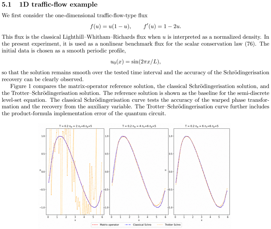
- The numerical experiments show that the Trotter\textendash{}Schr\"odingerisation circuit reproduces the reference evolution for a one-dimensional traffic-flow flux and a two-dimensional Burgers equation as the auxiliary resolution $N_w$ increases.
Reading between the lines
- The claimed advantage applies to observable estimation rather than full solution reconstruction; the paper itself notes that reading out all grid values would introduce a large measurement cost, and an end-to-end advantage would also require an efficient procedure for preparing the encoded initial state from $u_0$, which is assumed rather than constructed.
- A natural next test is to count the state-preparation and oracle-implementation circuits explicitly for a concrete flux such as Burgers, since those costs are excluded from the complexity comparison; if they scale with $N_x^d$, the polynomial-in-$d$ conclusion would be limited.
- The same level-set plus Schr\"odingerisation pipeline could plausibly extend to systems of conservation laws or Hamilton\textendash{}Jacobi equations, but the block-diagonal structure and flux-derivative loading become more involved there.
- The paper uses first-order Trotter formulas; higher-order product formulas would likely reduce the $T$ and $\varepsilon$ exponents in the gate count at the cost of more complicated controlled gates.
Editorial analysis
A structured set of objections, weighed in public.
Referee Report
Summary. The manuscript constructs an end-to-end quantum algorithm for scalar conservation laws by combining a level-set lifting to a linear Liouville equation, upwind finite-difference discretization, Schrödingerisation into a higher-dimensional Hamiltonian system, and explicit Trotterized circuits for the resulting evolution. It derives error bounds and gate-complexity estimates, with the main result in Theorem 2 stating that estimating an observable to precision ε costs eO(d^4 T^4 N_p N_w^2 ε^{-4}) gates, and Remark 5 uses this to claim a quantum advantage over classical finite-difference methods in sufficiently high spatial dimension. Numerical experiments for a one-dimensional traffic-flow flux and a two-dimensional Burgers equation, both with smooth data and before shock formation, are reported to validate accuracy and scaling.
Significance. If the algorithm computed the entropy solution of the scalar conservation law, the paper would be a valuable contribution: it gives an explicit circuit-level construction, imports and assembles Trotter error bounds in a coherent way, and improves the mollifier convergence by Richardson extrapolation. The use of the one-dimensional bounds from [21] as independent support for the p-multiplexed Hamiltonian is legitimate and not circular. However, the paper's central claim is compromised by a correctness gap in the shock regime: after wave breaking, the observable defined in Eq. (35) is a Jacobian-weighted average over all characteristic branches, and entropy selection conditions are absent. Since the numerical experiments are deliberately restricted to smooth solutions before shocks, they do not validate the claimed solution of the original nonlinear conservation law. The complexity result is also not yet an end-to-end bound because state preparation, oracle implementation, and measurement sampling are not costed. These issues are load-bearing for the claimed quantum advantage.
major comments (3)
- [Section 3.3, Eqs. (6) and (35)] The algorithm does not compute the entropy solution of the conservation law after shock formation. By Eq. (6), for multivalued times the level-set distribution is ψ(t,x,p)=Σ_ν |∂_p φ(p_ν)|^{-1}δ(p−p_ν), and Eq. (35) defines the recovered observable as ⟨G⟩_j = (1/N_p)Σ_l G(p_l)ψ_{j,l}(T), which is the Jacobian-weighted ensemble average over all characteristic branches. The entropy selection conditions (Rankine–Hugoniot and Oleinik conditions) do not appear anywhere in the algorithm, so this branch average is not G(u_entropy(T,x_j)). Consequently Theorem 2 bounds the cost of estimating an observable of the lifted multivalued problem, not of the original nonlinear scalar conservation law in the regime where shocks exist. The numerical experiments in Section 5 use smooth initial data and times before shock formation (Section 5.1 explicitly states that the solution remains smooth over the tested interval), so they do not test the regime in which the level-set method is needed. This is a load-bearing correctness gap for the paper's central claim of quantum advantage for nonlinear scalar conservation laws.
- [Section 3.2.2–3.2.3, Eqs. (21), (23), (24), (27)] The sign conventions in the Hermitian/skew-Hermitian decomposition and the Schrödingerised evolution are internally inconsistent. Equation (21) defines A_1 = (1/2)⊕_{α,l}(P^-_{α,l}−P^+_{α,l})(D_+−D_-) and A_2 = (1/(2i))⊕_{α,l}(P^-_{α,l}+P^+_{α,l})(D_++D_-). Equation (23) states ∂_t v̂ = i(ηA_1+A_2)v̂ = iH_C v̂, while Eq. (24) says d|v̂>/dt = −iH_C|v̂>. Equation (27) then sets U_C(τ)=exp(iH_Cτ). Moreover, the relative sign between H_1^{(l)} in Eq. (26) and β_{1,α,l} in Eq. (60) is not matched to the sign of P^-−P^+ in Eq. (21). As written, a reader cannot determine whether the circuit implements the intended Liouville evolution or its negative-time/adjoint version. Since the paper's contribution is an explicit gate-level implementation, these sign inconsistencies must be resolved before the complexity and correctness claims can be verified.
- [Appendix E and Remark 5] The stated total complexity in Theorem 2 does not account for the full end-to-end procedure. Appendix E counts only the Hamiltonian evolution gates from Lemma 4, and Remark 5 assumes that preparing the initial encoded state |Ψ(0)⟩ from u_0 and implementing the coefficient oracles are efficient. No circuit or cost estimate is given for preparing the amplitude-encoded mollified initial data over N_p N_x^d grid points, for implementing the value oracle O_η in Eq. (50), or for converting the postselected states in Eqs. (39) and (47) into a classical estimate of ⟨G⟩ to precision ε. If any of these costs scales with N_x^d or with the required number of measurement repetitions, the claimed exponential-in-d advantage over classical finite differences disappears. The paper should either provide explicit circuits and costs for these components or state the quantum-advantage conclusion as conditional on them throughout the theorem and remark.
minor comments (4)
- [Appendix D] The balancing statement at the end of Appendix D is inconsistent: from ω∼(dht)^{1/4}, the error estimate ω^2 + dht/ω^2 gives ε=O((dht)^{1/2}), not O((dht)^{1/4}) as written. The earlier balancing in Section 3.3 using ω=O(ε^{1/2}) and h=O(ε^2/(dT)) also differs from the Appendix D derivation and should be reconciled.
- [Eq. (31)] In the definition of V_1^{(l)}[s], the variable is written as a∈Z, but it should be s∈Z to match the subsequent usage V_1^{(l)}[−2^{n_w−1}] and V_1^{(l)}[2^m]; this is a typographical error, not a mathematical issue.
- [Appendix D, Part III] The line “≤Ch^{1/ω^2}” appears to be a typesetting error; the intended bound is O(h/ω^2), consistent with the local truncation error O(h∂_{xx}ψ).
- [Section 3.3, Eq. (38)] The zeroth-moment expression in Eq. (38) omits the explicit 1/√(N_p) normalization from the Hadamard transform in Eq. (37) and does not state the post-selection success probability; these factors are needed for a complete accounting of the measurement cost.
Circularity Check
No circularity: complexity claim is a genuine assembly of independent level-set, Schrödingerisation, and 1D-circuit error bounds.
full rationale
No circularity found. The derivation chain is: level-set lifting (3)-(6) -> upwind finite-difference discretization (10)-(12) -> Hermitian/skew decomposition and Schrödingerisation (21)-(26) -> explicit Trotterized circuits (28)-(31) -> Trotter and circuit error bounds (64)-(72) -> per-step and total gate counts (Lemmas 3-4, Theorem 2) -> comparison with a standard first-order finite-difference classical cost (Remark 5). Each link is an explicit equation or a cited external result. The only author-overlapping citation is [21] (Hu, Jin, Liu, Zhang), used for the 1D Trotter/circuit error estimates (64)-(65); the present paper reduces the d-dimensional p-block Hamiltonian to independent 1D tensor factors before applying it, so the cited bound does not assume the multi-dimensional or p-multiplexed result under proof. Under rule 4, this is independent support and does not raise the circularity score. The quantum-advantage claim is explicitly conditional on efficient state preparation and oracle access (Remark 5: 'Efficient state preparation and implementation of the required coefficient oracles are also assumed'), which is a stated hypothesis rather than a fitted input renamed as a prediction. A correctness caveat, not a circularity: in the multi-valued/shock regime, Eq. (35) is, by the paper's own statement, the Jacobian-weighted branch average of the level-set distribution rather than the entropy solution of (1); Theorem 2's complexity therefore bounds estimation of that defined observable. The paper also contains apparent arithmetic inconsistencies in the epsilon-exponents of Remarks 3 and 5, but those are correctness/consistency concerns, not circular reductions.
Assumptions & free parameters
free parameters (3)
- Mollifier width scaling ω =
O(ε^(1/4)) (Richardson-corrected kernel)
- p-grid spacing h_p (via N_p) =
N_p = Θ(ε^(-3/4)) in Remark 5
- Auxiliary Fourier truncation R and grid size N_w =
R=O(log ε^-1), N_w=O(ε^-1) for e^-|w|, O(ε^(-1/(k+1))) for C^k smoothing g(w)
assumptions (4)
- domain assumption Multi-valued solutions admit a finite-branch representation ψ(t,x,p)=Σ_ν |∂_p φ|^-1 δ(p-p_ν) (Eq. (6), from Lemma 9 of [1]).
- domain assumption The warped-phase initial profile v̂(0)=Ψ(0)⊗η with η_r=2/(η_r^2+1) and truncation w∈[-πR,πR] captures the continuous Fourier transform of e^-|w| with error e^-R and Fourier discretization error O(N_w^-1) (or better for smooth g).
- domain assumption State preparation of |Ψ(0)⟩ and the coefficient/value oracles have costs that are negligible compared with the evolution circuit.
- standard math The Lie-Trotter error bound accumulates linearly in the number of steps and the commutator norm satisfies ∥[H_{1,α}^{(l)}, H_{2,α}^{(l)}]∥ ≤ 2 β_max^2 n_x/R, as asserted in Section 4.1.
Cite this review
Pith. "Pith review of An Efficient Explicit Implementation of a Quantum Algorithm with Quantum Advantage for Nonlinear Scalar Conservation Laws." pith.science (2026). https://pith.science/paper/CHEW5JH6
@misc{pith2026260809675,
  author       = {Pith},
  title        = {Pith review of: An Efficient Explicit Implementation of a Quantum Algorithm with Quantum Advantage for Nonlinear Scalar Conservation Laws},
  year         = {2026},
  howpublished = {\url{https://pith.science/paper/CHEW5JH6}},
  note         = {Machine review of arXiv:2608.09675}
}
read the original abstract
Quantum algorithms for nonlinear partial differential equations remain challenging because nonlinear dynamics are not directly amenable to unitary quantum simulation. Building on the level-set formulation, we construct a quantum algorithm and provide an explicit gate-level implementation for solving scalar conservation laws. The nonlinear equation is first lifted to a linear Liouville equation, discretized by finite differences, and then embedded into a unitary evolution through Schr\"odingerisation. We further develop quantum procedures for estimating relevant observables from the evolved state. Error bounds and gate-complexity estimates are established for the complete algorithm. The resulting complexity comparison demonstrates a quantum advantage for observable estimation in sufficiently high spatial dimensions, under standard assumptions on state preparation and oracle access. Finally, numerical experiments validate the accuracy, multidimensional applicability, and predicted scaling of the proposed method.
Figures


Figures from the paper (1 more)

Reference graph
Works this paper leans on
-
[21]
Quantum circuits for partial differential equations via Schr¨ odingerisation,
J. Hu, S. Jin, N. Liu, and L. Zhang, “Quantum circuits for partial differential equations via Schr¨ odingerisation,”Quantum, vol. 8, p. 1563, 2024. 4.1, 4.1, 4.2, 6
work page 2024
-
[1]
Quantum algorithms for nonlinear partial differential equations,
S. Jin and N. Liu, “Quantum algorithms for nonlinear partial differential equations,”Bulletin des Sciences Math´ ematiques, vol. 194, p. 103457, 2024. (document), 1, 2.1, 5, 6 20
work page 2024
-
[2]
R. Courant and K. O. Friedrichs,Supersonic Flow and Shock Waves, ser. Applied Mathematical Sciences. New York: Springer-Verlag, 1976, vol. 21. 1
work page 1976
-
[3]
R. J. LeVeque,Finite Volume Methods for Hyperbolic Problems, ser. Cambridge Texts in Applied Math- ematics. Cambridge: Cambridge University Press, 2002. 1
work page 2002
-
[4]
On kinematic waves. II. a theory of traffic flow on long crowded roads,
M. J. Lighthill and G. B. Whitham, “On kinematic waves. II. a theory of traffic flow on long crowded roads,”Proceedings of the Royal Society of London. Series A. Mathematical and Physical Sciences, vol. 229, no. 1178, pp. 317–345, 1955. 1
work page 1955
-
[5]
Mechanism of fluid displacement in sands,
S. E. Buckley and M. C. Leverett, “Mechanism of fluid displacement in sands,”Transactions of the AIME, vol. 146, no. 1, pp. 107–116, 1942. 1
work page 1942
-
[6]
P. D. Lax,Hyperbolic Systems of Conservation Laws and the Mathematical Theory of Shock Waves, ser. CBMS–NSF Regional Conference Series in Applied Mathematics. Philadelphia: Society for Industrial and Applied Mathematics, 1973, vol. 11. 1
work page 1973
-
[7]
S. Jin and S. Osher, “A level set method for the computation of multi-valued solutions to quasi-linear hyperbolic PDEs and Hamilton–Jacobi equations,”Communications in Mathematical Sciences, vol. 1, no. 3, pp. 575–591, 2003. 1, 2.1
work page 2003
Show all 23 references
-
[8]
Efficient implementation of essentially non-oscillatory shock-capturing schemes,
C.-W. Shu and S. Osher, “Efficient implementation of essentially non-oscillatory shock-capturing schemes,”Journal of Computational Physics, vol. 77, no. 2, pp. 439–471, 1988. 1
1988
-
[9]
The Runge–Kutta discontinuous Galerkin method for conservation laws. V. multidimensional systems,
B. Cockburn and C.-W. Shu, “The Runge–Kutta discontinuous Galerkin method for conservation laws. V. multidimensional systems,”Journal of Computational Physics, vol. 141, no. 2, pp. 199–224, 1998. 1
1998
-
[10]
Universal quantum simulators,
S. Lloyd, “Universal quantum simulators,”Science, vol. 273, no. 5278, pp. 1073–1078, 1996. 1
1996
-
[11]
Simulating hamiltonian dynamics with a truncated Taylor series,
D. W. Berry, A. M. Childs, R. Cleve, R. Kothari, and R. D. Somma, “Simulating hamiltonian dynamics with a truncated Taylor series,”Physical Review Letters, vol. 114, no. 9, p. 090502, 2015. 1
2015
-
[12]
Optimal hamiltonian simulation by quantum signal processing,
G. H. Low and I. L. Chuang, “Optimal hamiltonian simulation by quantum signal processing,”Physical Review Letters, vol. 118, no. 1, p. 010501, 2017. 1
2017
-
[13]
Quantum simulation of partial differential equations via Schr¨ odingerization,
S. Jin, N. Liu, and Y. Yu, “Quantum simulation of partial differential equations via Schr¨ odingerization,” Physical Review Letters, vol. 133, no. 23, p. 230602, 2024. 1, 3.2.2
2024
-
[14]
Quantum simulation of partial differential equations: Applications and detailed analysis,
——, “Quantum simulation of partial differential equations: Applications and detailed analysis,”Phys- ical Review A, vol. 108, no. 3, p. 032603, 2023. 1
2023
-
[15]
Theory of Trotter error with commutator scaling,
A. M. Childs, Y. Su, M. C. Tran, N. Wiebe, and S. Zhu, “Theory of Trotter error with commutator scaling,”Physical Review X, vol. 11, no. 1, p. 011020, 2021. 1, 4.1
2021
-
[16]
Trotter error with commutator scaling for the Fermi–Hubbard model,
A. Schubert and C. B. Mendl, “Trotter error with commutator scaling for the Fermi–Hubbard model,” Physical Review B, vol. 108, no. 19, p. 195105, 2023. 1
2023
-
[17]
Quantum algorithm for nonlinear differential equations,
S. Lloyd, G. De Palma, C. G¨ okler, B. T. Kiani, Z.-W. Liu, M. Marvian, F. Tennie, and T. Palmer, “Quantum algorithm for nonlinear differential equations,” 2020, arXiv:2011.06571. 1
2020 arXiv
-
[18]
A quantum algorithm to solve nonlinear differential equations,
S. K. Leyton and T. J. Osborne, “A quantum algorithm to solve nonlinear differential equations,” 2008, arXiv:0812.4423. 1
2008 arXiv
-
[19]
Koopman–von Neumann approach to quantum simulation of nonlinear classical dynamics,
I. Joseph, “Koopman–von Neumann approach to quantum simulation of nonlinear classical dynamics,” Physical Review Research, vol. 2, no. 4, p. 043102, 2020. 1 21
2020
-
[20]
Hamiltonian simulation for hy- perbolic partial differential equations by scalable quantum circuits,
Y. Sato, R. Kondo, I. Hamamura, T. Onodera, and N. Yamamoto, “Hamiltonian simulation for hy- perbolic partial differential equations by scalable quantum circuits,”Physical Review Research, vol. 6, no. 3, p. 033246, 2024. 1, 3.1, 1, 3.2.3, 6
2024
-
[22]
Schr¨ odingerization based computationally stable algorithms for ill-posed problems in partial differential equations,
S. Jin, N. Liu, and C. Ma, “Schr¨ odingerization based computationally stable algorithms for ill-posed problems in partial differential equations,”SIAM Journal on Scientific Computing, vol. 47, no. 4, pp. B976–B1000, 2025. 3
2025
-
[23]
Unitarylab,
UnitaryLab Quantum Technology Co., Ltd., “Unitarylab,” 2026. 5 A The quantum circuits ofV 1(−τ) In this appendix, we provide the explicit construction of the quantum circuits for the operatorV 1(−τ), which approximates the evolutionU 1(−τ) = exp(−iH 1τ). Based on the Lie-Trott...
2026
Reviewed August 11, 2026 · model on record in the stance chip above.
Discussion (0). Continue with ORCID to comment.