Prediction in regression models with continuous observations

Anatoly Zhigljavsky; Andrey Pepelyshev; Holger Dette

REVIEW 1 major objections 6 minor 12 references

Prediction in regression models with continuous observations

T0 review · 1 major / 6 minor · reviewed 2026-08-14 · deepseek-v4-flash

Challenge this review Re-run · record.json Download PDF Read on arXiv ↗ Review JSON

Pith's one-line read The paper proves that continuous kriging has an exact best linear unbiased predictor, given by a signed measure that adds a covariance-matching term to the best linear unbiased estimator of the trend.

desk verdict A useful continuous-observation BLUP paper with one real overclaim about Assumption A; worth refereeing and publishing after a fix. read the letter →

arxiv 1908.04106 v1 pith:CM37ZJAB submitted 2019-08-12 math.ST stat.TH

Holger Dette , Andrey Pepelyshev , Anatoly Zhigljavsky This is my paper · ORCID

classification math.STstat.TH MSC 62M2060G25

keywords krigingbestlinearunbiasedpredictioncontinuousobservationssignedmeasuresintegralequationsreproducingkernelHilbertspaceMatérn3/2derivative

verification ladder T0 review T1 audit T2 compute T3 formal

The pith

A machine-rendered reading of the paper's core claim, the machinery that carries it, and where it could break.

The reading

This paper extends kriging—prediction of a random process from correlated observations—from finite sets of points to continuous observation regions. It proves that the best linear unbiased predictor exists and takes an explicit two-term form whenever two signed measures exist: one reproducing the target covariance and one defining the best unbiased trend estimator. The same machinery predicts derivatives and weighted averages, and the paper works out closed-form predictors for exponential, Matérn 3/2, and integrated-Brownian-motion kernels. A reader should care because the continuous formulas give exact benchmarks that discrete designs can be checked against, and they reveal when derivative observations are useless for prediction. The main theorem is Theorem 2.1, with generalizations in Theorems 2.2 and 3.1.

What carries the argument

The load-bearing object is the BLUP measure, a signed measure on the observation set that acts as the continuous analogue of the weight vector in classical kriging. Theorem 2.1 writes it as $\zeta_{t_0}(dt)+c^\top G(dt)$: the first term interpolates the residual covariance through equation (2.1), and the second term corrects the trend by adding the BLUE measure $G$ scaled by $c$. Assumption A is the existence condition: a signed matrix measure $G$ for the BLUE, and a signed measure $\zeta_{t_0}$ solving the covariance integral equation. Reproducing-kernel-Hilbert-space conditions make the assumption concrete, and for finite $T$ the whole construction reduces to the standard discrete kriging equations.

What would settle it

Compute the claimed continuous root-MSE for the location-scale model on $[0,1]$ with the Matérn 3/2 kernel at $t_0=2$ (0.9985569896 in Table 2) and compare it with a high-resolution discretization of the proposed predictor. If any signed continuous weighting achieves a strictly smaller mean squared error, Theorem 2.1 is not giving the true BLUP; equivalently, one can test Assumption A directly by checking whether equation (2.1) admits a signed-measure solution for a kernel whose section $K(t_0,\cdot)$ lies outside the reproducing kernel Hilbert space.

Watch

Extended reading notes

Core claim

The paper's central claim is that kriging with continuous observations has an exact solution, not merely a limit of discrete predictors. For a process $y(t)=f(t)^\top\theta+\varepsilon(t)$ observed at all $t$ in a set $T$, the best linear unbiased predictor of $y(t_0)$ is an integral against a signed measure $Q^*$, which splits as $Q^*(dt)=\zeta_{t_0}(dt)+c^\top G(dt)$. Here $G$ is the signed measure defining the best linear unbiased estimator of $\theta$, $\zeta_{t_0}$ solves the integral equation $\int_T K(t,s)\zeta_{t_0}(dt)=K(t_0,s)$, and $c=f(t_0)-\int_T f(t)\zeta_{t_0}(dt)$ enforces unbiasedness. The same representation covers prediction of a $p$th derivative and of weighted averages $\int_S y\,d\nu$, with the kernel section replaced by the appropriate derivative or averaged section. The proof shows that any competing unbiased predictor differs from $Q^*$ by a measure $R$ whose cross term vanishes, so $Q^*$ has minimal mean squared error.

Load-bearing premise

The load-bearing premise is that, for every prediction target, two exact signed weighting schemes exist—one that reproduces the covariance section $K(t_0,\cdot)$ by integrating $K(t,\cdot)$, and one that defines the best linear unbiased estimator of the trend—and if either is missing the formulas are not guaranteed.

Editorial extensions

If this is right

The discrete kriging formula reduces from the continuous theorem when $T$ is finite, so the continuous theory contains the standard formula as a special case.
Predicting a derivative $y^{(p)}(t_0)$ or a weighted average $\int_S y\,d\nu$ uses the same two-term structure, so a single implementation can switch among these targets by changing the covariance section.
For separable product kernels on rectangles, the BLUP measure factorizes into products of one-dimensional measures, reducing multivariate prediction to univariate integral equations.
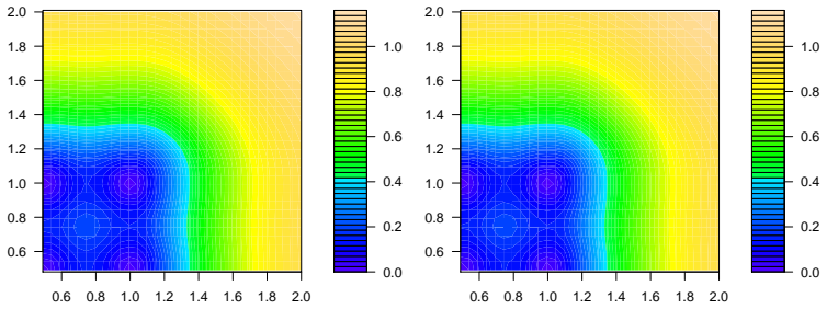
The numerical tables show that small discrete grids already nearly reach the continuous-observation MSE for the kernels studied, giving a practical benchmark for design.
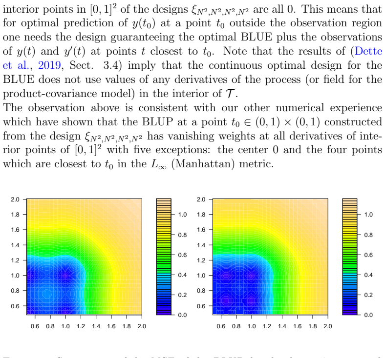
For the Matérn 3/2 and related kernels, derivative observations at interior points can receive zero weight when predicting outside the observation region, so those observations do not improve such predictions.

Reading between the lines

Editorial extensions of the paper, not claims the author makes directly.

The two-stage decomposition suggests a modular implementation: compute the BLUE measure once per model, then solve one integral equation per prediction target; the paper points to the shared BLUE part but does not develop the algorithmic consequences.
The observed zero-weight derivative phenomenon suggests a conjecture beyond the paper: for many kernels, an optimal prediction design is the BLUE-optimal design plus boundary information about the target point.
When Assumption A fails, a best linear unbiased predictor might still exist as a limit of discrete predictors; extending the theory to that case would require a more general existence argument.
The tables' continuous MSE values can serve as calibration targets: any discrete design reporting a lower MSE than the stated continuous value signals either a numerical error or a gap in the formula.

Share X Bluesky LinkedIn Reddit HN

Signed reviews

No signed human review yet.

Editorial analysis

A structured set of objections, weighed in public.

Desk editor's note, referee report, and a circularity audit.

Desk Editor's Note

read the letter

Dear colleague,

The paper gives exact BLUP formulas for continuous-observation regression, including derivative observations and weighted averages. That part is genuinely new and, given the assumptions, the proofs are clean. Theorem 2.1 and its generalization are correct as conditional statements; I checked the variational step and the algebra in Theorem 2.2's proof, and it holds.

The soft spot is Section 2.2. The claim 'If all components of f belong to HK then Assumption A holds' is false. The counterexample works: take K(t,s)=min(t,s) on [0,1], f(t)=t, t0=-1. Then f is in the RKHS, but (2.1) would require ∫ min(t,s)ζ(dt)=-1 for every s; evaluating at s=0 gives 0=-1. So no signed measure ζ_t0 exists. The general RKHS criterion is not sufficient. This is a real overclaim, and it matters because Assumption A is load-bearing for the main theorem. The paper does not characterize when ζ_t0 exists; it only verifies it in examples. That should be fixed, either with a correct sufficient condition or a candid statement that existence must be checked per kernel.

The examples are the best part. The Matérn 3/2 and OU cases are worked in detail, and those constructions do establish Assumption A for those kernels. The two-stage BLUE-plus-residual interpretation is useful and explains the computational savings. The numerical tables are consistent with the formulas. The heavy reliance on Dette et al. (2019) is justified because the BLUE is an ingredient, not a dodge.

Minor issues: dense notation, a few typos, and the tables would benefit from clear definitions of the designs. None of this changes the mathematics.

Who should read it? People working in kriging, computer experiments, or design of experiments who need continuous-domain predictors. It will likely become a standard reference for these formulas, once the sufficient condition is corrected.

I would send it to peer review. The conditional theorems are sound and the examples are valuable, but the Section 2.2 claim should be revised before publication. If an editor asked me, I'd accept after major revision rather than desk reject.

Referee Report

1 major / 6 minor

Summary. The paper studies best linear unbiased prediction for linear models y(t)=θ^T f(t)+ε(t) with correlated errors when the observation design is continuous, and it also covers prediction of weighted averages and of derivatives when derivative observations are available. The central results, Theorem 2.1 for point prediction, Theorem 2.2 for prediction of averages, and Theorem 3.1 for derivative observations, give explicit formulas for the BLUP measure Q* as a correction to a measure solving an integral equation involving the covariance kernel, plus a correction term involving the BLUE measure. The proofs are variational: they write the MSE as a quadratic form, define R=Q−Q*, use the unbiasedness condition to eliminate the trend term, and use nonnegative definiteness of the covariance kernel to show optimality. The paper also treats separable product kernels, derives explicit BLUPs for Markovian kernels, Brownian motion, Ornstein-Uhlenbeck processes, integrated Brownian motion, and the Matérn 3/2 kernel, and presents numerical tables comparing discrete designs with continuous designs.

Significance. Conditional on the assumptions, the paper provides a clean and useful framework for continuous-observation kriging, including derivative observations and prediction of weighted averages. The MSE decompositions and the two-stage interpretation in terms of the BLUE are natural and likely to be practically useful, and the explicit examples for popular kernels are valuable. The main proofs are transparent and the algebra checks out. The principal weakness is that the validation of the central Assumption A in Section 2.2 overclaims a general sufficient condition that is false; the examples in the appendix do verify the assumptions case by case, so the conditional theorems remain sound, but the generality claimed in the text needs correction.

major comments (1)

[Section 2.2] The asserted sufficient condition "If all components of f belong to H_K then Assumption A holds" is false as stated. Take T=[0,1], K(t,s)=min(t,s) (Brownian motion), f(t)=t, and t0=−1. The function f lies in the RKHS H_K because it is absolutely continuous with f(0)=0 and square-integrable derivative, and the first part of Assumption A holds: the measure G(dt)=δ_1(dt)−δ_0(dt) satisfies ∫ f(t)G(dt)=1 and ∫ K(t,s)G(dt)=s, so D=1. However, equation (2.1) would require ∫_0^1 min(t,s)ζ(dt)=min(−1,s)=−1 for every s∈[0,1], which is impossible because at s=0 the left-hand side is ∫_0^1 min(t,0)ζ(dt)=0. Thus Assumption A fails even though f∈H_K. This implication is load-bearing for the general applicability claim of Theorem 2.1, so the text should be rewritten either to remove the implication or to state correct, verifiable conditions under which the measure ζ_t0 solving (2.1) and the BLUE measure G exist.

minor comments (6)

[Section 4.1] The first line of Section 4.1, "To start, we proof the following lemma," should read "To start, we prove the following lemma."
[Section 3.3, Example 3.2] In the list of designs, item (iv) is assigned the same subscript ξ_{N^2,N^2,N^2,0} as item (iii), but its description and Table 3 indicate that it should be ξ_{N^2,4N−4,4N−4,4N−4}.
[Table 2] The sentence following Table 2, "the square root of the BLUB," contains a typo; it should be "the square root of the MSE of the BLUP."
[Table 3] The lower block of Table 3 repeats the row label ξ_{N^2,0,0,0} for the second target point; the table should clearly separate the two target points or relabel the rows to avoid ambiguity.
[Section 3.2, Assumption A''] The quantifier in equation (3.3), "∀s∈T_i," should be written as "for all s∈T_i, i=0,...,q," because the observation sets T_i are distinct and the equation must hold on each of them.
[Section 2.5] The notation T=(T1,T2) for the prediction point clashes with the notation T for the observation domain; using a lowercase symbol such as τ or t0 would improve readability.

Circularity Check

0 steps flagged · score 0.0 of 10

No circularity found; the BLUP theorem is conditional on explicit assumptions and its proof is self-contained, with prior BLUE results serving as independent external support.

full rationale

The paper's central results (Theorems 2.1, 2.2, and 3.1) are derived from explicit assumptions: existence of a BLUE measure G and of signed measures satisfying the integral equations (2.1), (2.9), or (3.3). The proofs do not assume the predictor they set out to construct; they decompose an arbitrary unbiased predictor into Q* plus a residual R and show the residual increases MSE using positivity of the covariance kernel and unbiasedness. The BLUP measure Q* is not defined through G and zeta; rather it is expressed in terms of them after a genuine minimization argument. The heavy citation of Dette et al. (2019) supplies the existence and form of the BLUE measure in examples; that is an external published theorem with its own proof and assumptions, not a restatement of this paper's target results, so it does not make the derivation circular. The discrete-observation match in Section 2.3 is a consistency check, not an input. No fitted parameters are renamed as predictions; kernel parameters such as lambda are fixed inputs, and the tables evaluate closed-form MSE expressions. The Section 2.2 sufficiency claim that Assumption A holds whenever the regression functions lie in the RKHS appears overbroad and has been challenged with a Brownian-motion counterexample, but that is a correctness/accuracy concern about Assumption A's validation, not a circularity: the main theorems remain conditional on Assumption A and do not feed their conclusions back into their hypotheses.

Assumptions & free parameters 0 free parameters · 6 assumptions · 0 invented entities

The paper introduces no fitted parameters and no new entities. Its results rest on the standard linear model with a covariance kernel, positive definiteness and smoothness conditions, and the existence assumptions A/A'/A'' for the BLUE and the integral-equation measures. The latter are regularity conditions, not free parameters.

assumptions (6)

domain assumption The response follows the linear model y(t) = f^T(t)θ + ε(t) with zero-mean correlated error having covariance kernel K(t,s).
Core model (1.1) underlying all results.
domain assumption The covariance kernel K is strictly positive definite.
Stated in Section 2.1 before Theorem 2.1; ensures invertibility of covariance operators.
domain assumption The regression functions in f are bounded, integrable, smooth enough, and linearly independent on T.
Stated in Section 2.1; needed for unbiasedness conditions.
domain assumption Assumption A/A'/A'': a BLUE exists and a signed measure solving the relevant integral equation (2.1)/(2.9)/(3.3) exists.
This is the central regularity condition; the paper does not prove it in general but verifies it for specific kernels via prior work and RKHS theory.
domain assumption For derivative prediction, the kernel K and f are q times differentiable and the process is q times differentiable in mean-square sense.
Section 3.2; required for the derivative observations and predictions.
standard math Parzen (1961) RKHS duality: if K(t0,·) belongs to H_K, then a measure ζ_t0 solving (2.1) exists.
Used in Section 2.2 to justify Assumption A.

how reviews work

0 comments

Cite this review

Pith. "Pith review of Prediction in regression models with continuous observations." pith.science (2026). https://pith.science/paper/CM37ZJAB

@misc{pith2026190804106,
  author       = {Pith},
  title        = {Pith review of: Prediction in regression models with continuous observations},
  year         = {2026},
  howpublished = {\url{https://pith.science/paper/CM37ZJAB}},
  note         = {Machine review of arXiv:1908.04106}
}

abstract

We consider the problem of predicting values of a random process or field satisfying a linear model $y(x)=\theta^\top f(x) + \varepsilon(x)$, where errors $\varepsilon(x)$ are correlated. This is a common problem in kriging, where the case of discrete observations is standard. By focussing on the case of continuous observations, we derive expressions for the best linear unbiased predictors and their mean squared error. Our results are also applicable in the case where the derivatives of the process $y$ are available, and either a response or one of its derivatives need to be predicted. The theoretical results are illustrated by several examples in particular for the popular Mat\'{e}rn $3/2$ kernel.

Figures

Figures reproduced from arXiv: 1908.04106 by the authors.

**Figure 1.** The square root of the MSE of the BLUP for the N ×N-point equidistant design with N = 3 (left) and N = 4 (right) and the exponential kernel with λ = 2. model (1.1). For the process y to be q times differentiable, the covariance kernel K and vector-function f in (1.1) have to be q times differentiable, which is one of the assumptions in Section 3.2. In Section 3.3 we consider the prediction problem for the location s… view at source ↗

**Figure 2.** Square root of the MSE of the BLUP for the design ξN2,0,0,0 with N = 3 (left) and N = 4 (right), and the Mat´ern 3/2 product-kernel with λ = 2. Figures 2 and 3 compare the MSE for some designs. As [PITH_FULL_IMAGE:figures/full_fig_p020_2.png] view at source ↗

**Figure 3.** Square root of the MSE of the BLUP for the design ξN2,4N−4,4N−4,4N−4 (left) and ξN2,N2,N2,N2 (right) with N = 3 and the Mat´ern 3/2 product-kernel with λ = 2. 4 Proofs 4.1 Proof of Theorem 2.2 To start, we proof the following lemma. Lemma 4.1. The mean squared error [relative to the true process value] of any unbiased estimator ZˆQ = R T y(t)Q(dt) is given by MSE(ZˆQ) = E Z − ZˆQ 2 = Z S Z S K(t, s)ν(dt)ν(ds)−2 Z… view at source ↗

Discussion (0). Continue with ORCID to comment.

Reference graph

Works this paper leans on

12 extracted references · 12 canonical work pages

[1]

Statistics for Spatial Data

Cressie, N., 1993. Statistics for Spatial Data. John Wiley & Sons

work page 1993
[2]

The blue in continuous- time regression models with correlated errors

Dette, H., Pepelyshev, A., Zhigljavsky, A., 2019. The blue in continuous- time regression models with correlated errors. Annals of Statistics 47, 1928–1959

work page 2019
[3]

Testing for separability of spatial-temporal covariance functions

Fuentes, M., 2006. Testing for separability of spatial-temporal covariance functions. Journal of Statistical Planning and Inference 136 (2), 447–466

work page 2006
[4]

Geostatistical space-time models, stationarity, separability and full symmetry

Gneiting, T., Genton, M., Guttorp, P., 2007. Geostatistical space-time models, stationarity, separability and full symmetry. In: B. Finkenstadt, 28 L. Held, V. I. (Ed.), Statistical Methods for Spatio-temporal Systems. Chapman and Hall / CRC, Boca Raton, FL, pp. 151–176

work page 2007
[5]

R., Dean, A

Leatherman, E. R., Dean, A. M., Santner, T. J., 2017. Designing combined physical and computer experiments to maximize prediction accuracy. Com- putational Statistics & Data Analysis 113, 346–362

work page 2017
[6]

D., Mitchell, T

Morris, M. D., Mitchell, T. J., Ylvisaker, D., 1993. Bayesian design and analysis of computer experiments: use of derivatives in surface prediction. Technometrics 35 (3), 243–255. N¨ ather, W.,ˇSim´ ak, J., 2003. Eﬀective observation of random processes using derivatives. Metrika 58 (1), 71–84

work page 1993
[7]

An approach to time series analysis

Parzen, E., 1961. An approach to time series analysis. The Annals of Math- ematical Statistics 32 (4), 951–989

work page 1961
[8]

Gaussian Processes for Machine Learning

Rasmussen, C., Williams, C., 2006. Gaussian Processes for Machine Learning. MIT Press

work page 2006

Show all 12 references

[9]

D., 1991

Ripley, B. D., 1991. Statistical Inference for Spatial Processes. Cambridge University Press

1991
[10]

J., Mitchell, T

Sacks, J., Welch, W. J., Mitchell, T. J., Wynn, H. P., 1989. Design and analysis of computer experiments. Statistical Science 4, 409–423

1989
[11]

J., Williams, B

Santner, T. J., Williams, B. J., Notz, W. I., 2003. The Design and Analysis of Computer Experiments. Springer Series in Statistics. New York: Springer- Verlag

2003
[12]

L., 1999

Stein, M. L., 1999. Interpolation of Spatial Data: Some Theory for Kriging. Springer Science & Business Media. 29

1999

Pith tools

Reviewed August 14, 2026 · model on record in the stance chip above.

[1] [1]

Statistics for Spatial Data

Cressie, N., 1993. Statistics for Spatial Data. John Wiley & Sons

work page 1993

[2] [2]

The blue in continuous- time regression models with correlated errors

Dette, H., Pepelyshev, A., Zhigljavsky, A., 2019. The blue in continuous- time regression models with correlated errors. Annals of Statistics 47, 1928–1959

work page 2019

[3] [3]

Testing for separability of spatial-temporal covariance functions

Fuentes, M., 2006. Testing for separability of spatial-temporal covariance functions. Journal of Statistical Planning and Inference 136 (2), 447–466

work page 2006

[4] [4]

Geostatistical space-time models, stationarity, separability and full symmetry

Gneiting, T., Genton, M., Guttorp, P., 2007. Geostatistical space-time models, stationarity, separability and full symmetry. In: B. Finkenstadt, 28 L. Held, V. I. (Ed.), Statistical Methods for Spatio-temporal Systems. Chapman and Hall / CRC, Boca Raton, FL, pp. 151–176

work page 2007

[5] [5]

R., Dean, A

Leatherman, E. R., Dean, A. M., Santner, T. J., 2017. Designing combined physical and computer experiments to maximize prediction accuracy. Com- putational Statistics & Data Analysis 113, 346–362

work page 2017

[6] [6]

D., Mitchell, T

Morris, M. D., Mitchell, T. J., Ylvisaker, D., 1993. Bayesian design and analysis of computer experiments: use of derivatives in surface prediction. Technometrics 35 (3), 243–255. N¨ ather, W.,ˇSim´ ak, J., 2003. Eﬀective observation of random processes using derivatives. Metrika 58 (1), 71–84

work page 1993

[7] [7]

An approach to time series analysis

Parzen, E., 1961. An approach to time series analysis. The Annals of Math- ematical Statistics 32 (4), 951–989

work page 1961

[8] [8]

Gaussian Processes for Machine Learning

Rasmussen, C., Williams, C., 2006. Gaussian Processes for Machine Learning. MIT Press

work page 2006