REVIEW 1 major objections 4 minor 24 references
Expectile based measures of skewness
T0 review · 1 major / 4 minor · reviewed 2026-08-14 · deepseek-v4-flash
Pith's one-line read Expectile ratios define a skewness measure that is bounded, exists for all finite-mean distributions, and is zero exactly for symmetric ones.
desk verdict Solid, useful paper on expectile-based skewness; the main asymptotic variance formula has a factor-of-two error that needs fixing before it can be used as stated. read the letter →
The pith
A machine-rendered reading of the paper's core claim, the machinery that carries it, and where it could break.
The reading
What carries the argument
The central object is the expectile skewness family $s_2(\alpha)$, a normalized ratio of the expectile deviations $e_X(1-\alpha)-\mu$ and $\mu-e_X(\alpha)$. The expectile $e_X(\alpha)$ is the minimizer of the asymmetric quadratic loss $\alpha E[(X-t)_+^2]+(1-\alpha)E[(X-t)_-^2]$, acting as a smoothed quantile and making the ratio sensitive to the whole distribution. The companion skewness function is $S_X(t)=\frac{1}{t}\{\pi_X(\mu+t)-\pi_X(\mu-t)\}+1$, expressed through the stop-loss transform $\pi_X(t)=E(X-t)_+$ and the $\Omega$ ratio $\Omega_X(t)=E(X-t)_+/E(X-t)_-$; its scale-invariant version $\tilde{S}_X(t)=S_X(t\delta_X)$ carries the convex-order comparison in Theorem 9.
What would settle it
Draw many samples from a skewed distribution with finite mean but infinite variance, such as a Pareto distribution with shape between 1 and 2, compute $\hat{s}_{2,n}(\alpha)$ and its nominal 95% confidence intervals using $\hat{\sigma}_\alpha$, and check whether the empirical coverage stays near 0.95; a large shortfall would show that the normal limit in Theorem 11 does not cover the motivating heavy-tailed case.
Extended reading notes
Core claim
The paper's central claim is that the expectile function $e_X(\alpha)$, defined by minimizing asymmetric quadratic loss, encodes skewness in a normalized ratio of upper and lower deviations from the mean. A distribution is symmetric exactly when $e_X(1-\alpha)-\mu = \mu-e_X(\alpha)$ for all $\alpha\in(0,1/2)$; the family $s_2(\alpha)$ turns that condition into a bounded scalar between $-1$ and $1$. The paper proves that $s_2$ is location- and scale-invariant, derives its limiting value $s_3=2F(\mu)-1$, and establishes that the plug-in estimator $\hat{s}_{2,n}(\alpha)$ is strongly consistent under $E|X|<\infty$ and asymptotically normal with explicit variance under $EX^2<\infty$ when the distribution has no point mass at the relevant expectiles. For the companion scale-invariant skewness function $\tilde{S}_X(t)$, it proves monotonicity with respect to a skewness order that is weaker than the convex transformation order but stronger than a known weak skewness order.
Load-bearing premise
The asymptotic normality results require a finite second moment and no point mass exactly at the expectiles being used; when that fails, the practical confidence intervals are not justified, and only consistency under a finite mean remains.
Editorial extensions
If this is right
- Skewness can be estimated and compared for heavy-tailed distributions with finite mean, where the classical moment measure is unstable or undefined.
- Asymptotic confidence intervals for $s_2(\alpha)$ follow from the delta method under a finite second moment, avoiding the density estimation needed for quantile-based skewness.
- The limiting value $s_3=2F(\mu)-1$ links the family to the sign-test statistic and gives a parameter-free representative of $s_2(\alpha)$ near $\alpha=1/2$.
- The scale-invariant function $\tilde{S}_X$ is monotone under the convex transformation order, so comparisons of skewness agree with a standard stochastic ordering of distributions.
Reading between the lines
- If the paper's conjecture that $s_2$ itself satisfies van Zwet's convex-order property (S3) is confirmed, the family would inherit the strongest standard skewness-ordering guarantee rather than only its limiting case.
- Because $s_2(\alpha)$ is a smooth functional of the whole expectile curve, scanning a grid of $\alpha$ values could detect skewness concentrated in particular regions of the distribution, a feature quartile-based measures miss.
- The finite-variance requirement for asymptotic normality suggests a bootstrap or heavy-tailed central-limit extension would be needed to justify confidence intervals for very heavy-tailed data; the paper's own consistency result is weaker.
- The connection to Omega ratios means the same construction could be imported directly into portfolio performance and risk measurement, where Omega ratios are already standard.
Signed reviews
Editorial analysis
A structured set of objections, weighed in public.
Referee Report
Summary. The paper introduces a family of expectile-based skewness measures, primarily s2(α) = (e_X(1−α)+e_X(α)−2μ) / ((1−2α)(e_X(1−α)−e_X(α))), and studies their theoretical and empirical properties. The authors show that these measures are normalized on (−1,1) with sharp bounds, characterize symmetry, are linked to Omega ratios and stop-loss transforms, and that a scale-invariant skewness function preserves the convex transformation order. They also derive plug-in estimators, prove strong consistency and asymptotic normality, provide an explicit asymptotic variance formula, and compare the new measures with quantile-based and moment-based skewness in simulations.
Significance. If the results are correct, the paper makes a useful contribution to the skewness-measurement literature: the expectile-based family avoids the heavy-tail sensitivity of the third central moment, is fully defined for finite-mean distributions, characterizes symmetry, and has convenient asymptotic inference without density estimation. The connection to Tajuddin's s3 as a limiting case, the sharp bounds in Proposition 4, and the ordering result in Theorem 9 are valuable. The paper also includes explicit proofs and a simulation study. The main mathematical claims are plausible and largely well supported, but the asymptotic variance in Theorem 11 contains an algebraic error that needs correction before the inference results can be used.
major comments (1)
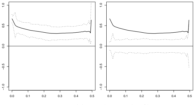
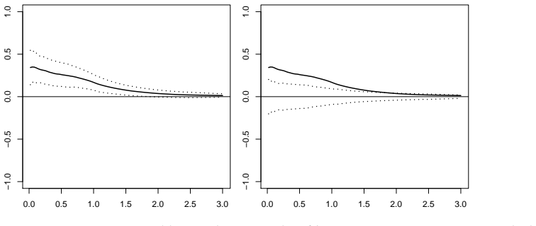
- [Theorem 11 and Eq. (19)] The displayed formula for σα^2 in Theorem 11 is missing a factor 2 in the covariance term between the two expectile estimators. Let L=e_X(α), U=e_X(1−α), D=U−L, c=1−2α, and S(τ)=τ+(1−2τ)F(e_X(τ)). The gradient of s2 with respect to (L,U,μ) is (2(U−μ)/(cD^2), 2(μ−L)/(cD^2), −2/(cD)). Using the notation A(α)=(U−μ)/S(α) and A(1−α)=(μ−L)/S(1−α), the covariance contribution between the two expectiles is 2·(2A(α)S(α)/(cD^2))·(2A(1−α)S(1−α)/(cD^2))·η(α,1−α)/(S(α)S(1−α)) = 8A(α)A(1−α)η(α,1−α)/(c^2D^4). After factoring out 4/c^2, the bracket must contain 2A(α)A(1−α)η(α,1−α), not A(α)A(1−α)η(α,1−α). As a consequence, the plug-in variance estimator and the confidence intervals (19) and (20) are mis-sized if the displayed formula is taken literally. The asymptotic normality itself remains valid; the fix is local, but it is load-bearing for the paper's inference contribution.
minor comments (4)
- [Section 5.1, after Theorem 13] The definition of p̂_t uses the true mean μ in the indicator 1_{μ−t<X_i≤μ+t}, while the displayed expression for σ̂_t^2 uses X_i−X̄ alongside p̂_t. For a genuine plug-in estimator, p̂_t should be defined with X̄ in place of μ.
- [Section 3.1] In Remark 10.2, the phrase 'the limiting measure s3(α)' is misleading because s3 does not depend on α; this should be simply s3.
- [Section 6.1] There is a typo: 'decrasing' should be 'decreasing'.
- [References] In the reference to Bellini, Klar, and Müller (2018), the umlaut is missing ('Mller' should be 'Müller').
Circularity Check
No significant circularity: definitions are explicit, derivations are self-contained, and the cited expectile asymptotics are external published results.
full rationale
The paper proposes new definitions rather than fitting parameters and relabeling them as predictions. Definition 3 defines expectile right-skewness by inequality (6), and s2 in (8) is the normalized difference of the two sides of that inequality; the sign characterization is immediate by construction, but this is an explicit definition and not a disguised reuse of the target result. Proposition 4 derives the attainable range of s2 from the expectile first-order condition (5), with sharpness shown by Bernoulli examples. Theorem 9's ordering property is proved from crossing-count arguments and the integral identities (29)-(32), not assumed. The main external input is the asymptotic normality of finitely many empirical expectiles from Holzmann and Klar (2016); although Bernhard Klar is a co-author of that paper, it is a published, parameter-free theorem whose stated assumptions (finite second moment, no point mass at the expectiles) do not include the target results of this paper, so it functions as independent evidence and does not constitute circularity. No fitted input is called a prediction: the plug-in estimators in Section 5 are obtained by replacing expectiles with empirical expectiles, and the asymptotic variances are computed by the delta method. The paper explicitly leaves property S3 for s2 as an open question (Remark 10.2), so no unsupported claim is smuggled. The reviewer-flagged possible factor-of-2 error in Theorem 11's variance formula, if valid, would be a numerical correctness issue rather than a circularity step.
Assumptions & free parameters
assumptions (6)
- domain assumption All random variables are assumed non-degenerate and to have finite first moment, X in L1.
- standard math The expectile properties in Proposition 1 (translation equivariance, scale equivariance, monotonicity, derivative formula) are taken from Newey and Powell (1986) and Bellini et al. (2014).
- standard math Asymptotic normality of finite-dimensional empirical expectiles is taken from Holzmann and Klar (2016) and combined with the delta method.
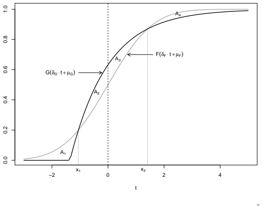
- domain assumption For the ordering results in Theorem 9, cdfs are absolutely continuous and strictly increasing, and Oja's crossing characterization of the convex transform order is used.
- domain assumption Theorem 11 assumes EX^2 is finite and that F has no point mass at e_X(alpha), e_X(1/2), or e_X(1-alpha).
- domain assumption For s3 to satisfy property S2, the paper assumes P(X = mu) = 0.
Cite this review
Pith. "Pith review of Expectile based measures of skewness." pith.science (2026). https://pith.science/paper/CRIN5TRQ
@misc{pith2026190808243,
  author       = {Pith},
  title        = {Pith review of: Expectile based measures of skewness},
  year         = {2026},
  howpublished = {\url{https://pith.science/paper/CRIN5TRQ}},
  note         = {Machine review of arXiv:1908.08243}
}
read the original abstract
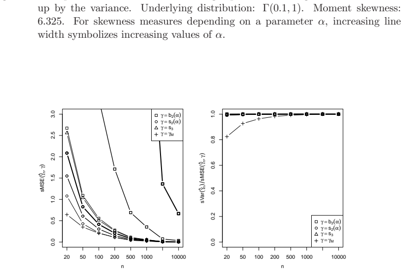
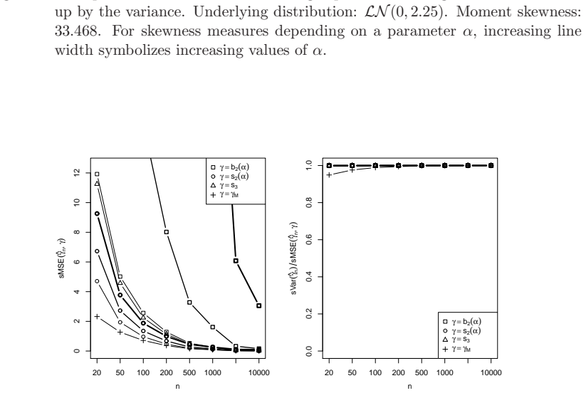
In the literature, quite a few measures have been proposed for quantifying the deviation of a probability distribution from symmetry. The most popular of these skewness measures are based on the third centralized moment and on quantiles. However, there are major drawbacks in using these quantities. These include a strong emphasis on the distributional tails and a poor asymptotic behaviour for the (empirical) moment based measure as well as difficult statistical inference and strange behaviour for discrete distributions for quantile based measures. Therefore, in this paper, we introduce skewness measures based on or connected with expectiles. Since expectiles can be seen as smoothed versions of quantiles, they preserve the advantages over the moment based measure while not exhibiting most of the disadvantages of quantile based measures. We introduce corresponding empirical counterparts and derive asymptotic properties. Finally, we conduct a simulation study, comparing the newly introduced measures with established ones, and evaluating the performance of the respective estimators.
Figures

Figures from the paper (8 more)



Reference graph
Works this paper leans on
-
[1]
Arnold, B. C., Groeneveld, R. A., 1993. Skewness and kurtosis orderings: an introduction. Stochastic inequalities, IMS Lecture Notes - Monograph Series , 22, 1993, 17--24
work page 1993
- [2]
-
[3]
Bellini, F. (2012). Isotonicity results for generalized quantiles. Statistics and Probability Letters 82, 2017-2024
work page 2012
-
[4]
Bellini, F., Klar, B., M\" u ller, A., Rosazza Gianin, E. (2014). Generalized quantiles as risk measures. Insurance: Mathematics and Economics 54, 41-48
work page 2014
-
[5]
Bellini, F., Klar, B., Müller, A. (2018). Expectiles, Omega Ratios and Stochastic Ordering. Methodology and Computing in Applied Probability 20, 855–873
work page 2018
-
[6]
Benjamini Y., Krieger, A.M. (1996). Concepts and Measures for Skewness with Data-Analytic Implications. The Canadian Journal of Statistics 24, 131-140
work page 1996
-
[7]
Bowley, A.L. (1920). Elements of Statistics , 4th edn. Charles Scribner's Sons, New York
work page 1920
-
[8]
Critchley, F., Jones, M.C. (2008). Asymmetry and gradient asymmetry functions: density-based skewness and kurtosis. Scand. J. Stat. 35, 415-437
work page 2008
Show all 24 references
-
[9]
David, F.N., Johnson, N.L. (1956). Some tests of significance with ordered variables. J. R. Stat. Soc. Ser. B Stat. Methodol. 18, 1–31
1956
-
[10]
Gastwirth, J.L. (1971). On the Sign Test for Symmetry. Journal of the American Statistical Association 66, 821-823
1971
-
[11]
Groeneveld, R.A., Meeden, G. (1984). Measuring Skewness and Kurtosis. Journal of the Royal Statistical Society. Series D (The Statistician) 33, 391-399
1984
-
[12]
Hinkley, D.V. (1975). On power transformations to symmetry. Biometrika 62, 101–111
1975
-
[13]
Hosking, J.R.M. (1990). L-moments: Analysis and estimation of distributions using linear combinations of order statistics. Journal of the Royal Statistical Society. Series B (Methodological) 52, 105-124
1990
-
[14]
Holzmann, H., Klar, B. (2016). Expectile Asymptotics. Electronic Journal of Statistics 10, 2355-2371
2016
-
[15]
Keating, C., Shadwick, W. F. (2002). A Universal Performance Measure. The Finance Development Centre, London
2002
-
[16]
L., 1986
MacGillivray, H. L., 1986. Skewness and Asymmetry: Measures and Orderings. The Annals of Statistics , 14, 994--1011
1986
-
[17]
M\" u ller, A. (1996). Ordering of risks: A comparative study via stop-loss transforms. Insurance: Mathematics and Economics 17, 215-222
1996
-
[18]
M\" u ller, A., Stoyan, D. (2002). Comparison Methods for Stochastic Models and Risks. John Wiley & Sons Ltd., Chichester
2002
-
[19]
Newey, K., Powell, J. (1986). Asymmetric least squares estimation and testing. Econometrica 55, 819-847
1986
-
[20]
Oja, H. (1981). On Location, Scale, Skewness and Kurtosis of Univariate Distributions. Scandinavian Journal of Statistics , 8, 154--168
1981
-
[21]
Remillard, B. (2013). Statistical Methods for Financial Engineering. Chapman and Hall/CRC
2013
-
[22]
Tajuddin, I.H. (1999). A Comparison between Two Simple Measures of Skewness. Journal of Applied Statistics 26, 767-774
1999
-
[23]
Yule, G.U. (1912). An Introduction to the Theory of Statistics , 1st edn. Charles Griffin and Co, London
1912
-
[24]
Zwet, W. R. van (1964). Convex Transformations of Random Variables. Math. Centrum, Amsterdam
1964
Reviewed August 14, 2026 · model on record in the stance chip above.
Discussion (0). Continue with ORCID to comment.