REVIEW 3 major objections 4 minor 5 references
Quantum Path Signatures
T0 review · 3 major / 4 minor · reviewed 2026-08-05 · deepseek-v4-flash
Pith's one-line read Randomised unitary path developments satisfy a nonlocal loop equation, and in the Gaussian case a one-clean-qubit circuit estimates the resulting kernel efficiently.
desk verdict Worth a look: new loop equations for perturbed matrix models and a Pauli-ensemble convergence result are solid; the DQC1 algorithm's complexity proof has a real but fixable parameter-scaling error. read the letter →
The pith
A machine-rendered reading of the paper's core claim, the machinery that carries it, and where it could break.
The reading
What carries the argument
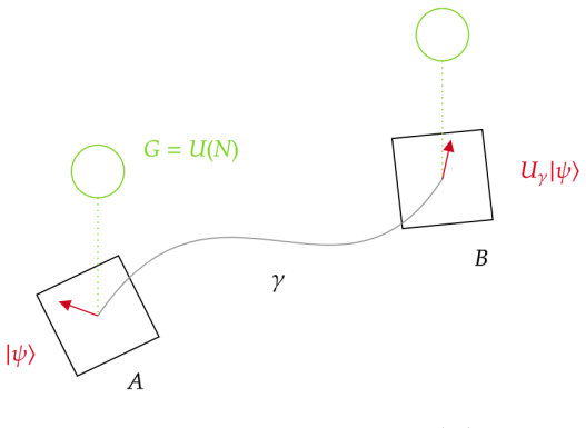
The central object is the randomised unitary path development, $U_{s,t}=\mathcal{P}\exp(i\sum_j A_j\,d\gamma^j)$, where $(A_1,\dots,A_d)$ are drawn from the matrix-model measure $\exp(-N\operatorname{tr}V(A))\,\mathrm{d}A$; its normalised trace, taken to $N=\infty$, is $\langle\gamma_{s,t}\rangle$. The argument is carried by two identities working together: the Schwinger-Dyson equation $\tau_V\otimes\tau_V(\partial_k P)=\tau_V(P D_k V)$, which fixes the non-commutative law of the matrix entries, and the vertical derivative $\nabla_w$ on path space, which turns coefficients of the signature into increments of $d\gamma$. In the algorithmic half, the load-bearing mechanism is the random Pauli e
What would settle it
Compute both sides of (39) for a straight-line path $\gamma_t=tv$ with a one-dimensional potential $V(X)=\frac12X^2+gX^4$, expanding in powers of $v$; the coefficients of the left side are determined by the moments $\tau_V(X^n)$, and the right side by the same moments through the Schwinger-Dyson equation. A mismatch at any order would disprove Theorem 3.14; alternatively, implement the circuit of Definition 4.9 with parameters as in the proof of Theorem 4.11 and compare the estimator against a classical Monte Carlo GUE average for a nontrivial path, checking the claimed $\epsilon,\delta$ guara
Extended reading notes
Core claim
The central claim of Section 3 is Theorem 3.14: writing $\langle\gamma_{s,t}\rangle_{\mu^\infty_V}$ for the large-$N$ limit of the expected normalised trace of the unitary development $U_{s,t}=\mathcal{P}\exp(i\sum_j\int A_j\,d\gamma^j)$ under the Gaussian-perturbed matrix-model measure, one has $$\langle\gamma_{s,t}\rangle = 1 - \int_{s\le u\le v\le t}\langle\gamma_{s,u}\rangle\langle\gamma_{u,v}\rangle\,\langle d\gamma_u,d\gamma_v\rangle - \sum_{k=1}^d\int_s^t D_k^W\langle\gamma_{s,u}\rangle\,d\gamma^k_u ,$$ with $\langle\gamma_{s,s}\rangle=1$. The derivation uses the signature expansion of the path-ordered exponential, identifies the large-$N$ moments with the non-commutative law $\tau_V$
Load-bearing premise
The load-bearing premise is the imported convergence theorem for the matrix-model measure: for a self-adjoint potential whose perturbation satisfies a convexity condition and has sufficiently small coupling coefficients, the large-N law converges to the unique Schwinger-Dyson solution with sub-Gaussian tails; if that fails for the chosen potential, the derivation of the loop equation collapses.
Editorial extensions
If this is right
- Every GUE signature kernel $k_{\mathrm{GUE}}(\sigma,\tau)$ can be evaluated as a single development $\langle\gamma\rangle$ with $\gamma=\sigma\star\overleftarrow{\tau}$, so the quantum algorithm directly estimates kernels from path increments.
- The loop equation (39) gives a new family of path-dependent observables in matrix models, interpolating between zero-dimensional QFT and Wilson lines, and reduces to the known spectral-curve loop equation for straight paths.
- For the Gaussian case, the quantum path signature $\mathcal{S}^Q(\gamma)=\mathbb{E}_{\alpha(m)}[U^Q_\gamma|0\rangle\langle0|U^{Q\dagger}_\gamma]$ is a well-defined feature map into the space of density matrices on $n$ qubits.
- The resource counts of Theorem 4.11—logarithmic in $1/\epsilon$ for space, polynomial in $1/\epsilon$ for gates—contrast with the classical algorithm of Theorem 4.12, whose matrix dimension must scale as $e^{2\Delta_\gamma}/\epsilon^2$; this is the concrete cost comparison the paper establishes.
- Within the class of infinite linear functionals on signatures, the solution of the loop equation is unique, so the limiting kernel is not an artifact of the expansion order.
Reading between the lines
- Editorial inference: the same Schwinger-Dyson-plus-vertical-derivative scheme should produce $1/N$ corrections to $\langle\gamma_{s,t}\rangle$ by applying topological recursion to path-loop correlators; the paper points at this as future work, so the concrete conjecture is that a genus expansion exists with the same structure as the standard matrix-model expansion.
- Editorial inference: because Theorem 4.8 is proved from moment bounds, one could replace the Gaussian law by any matrix-model potential whose limiting law satisfies the Schwinger-Dyson equation and sample a sparse Pauli ensemble with matching moments; the paper does not do this.
- Editorial inference: if the algorithm is run on a real device, the one-clean-qubit scheme tolerates a very impure 'clean' qubit; the analysis here assumes ideal gates, so a natural stress test is to add depolarising noise to the Pauli rotations and observe how the $\epsilon$ guarantee degrades.
Editorial analysis
A structured set of objections, weighed in public.
Referee Report
Summary. The paper develops a QFT/matrix-model perspective on path signatures, interpreting randomized path developments as Wilson lines and deriving a large-N integro-differential equation for the expected trace under Gaussian-perturbed matrix model potentials (Theorem 3.14), with a uniqueness result among linear signature functionals (Proposition 3.17). In the Gaussian case, the authors introduce a random Pauli-string ensemble, prove closeness of the resulting path development to the GUE development (Theorem 4.8), define a quantum path signature feature map via a Trotterized random quantum circuit, and give a one-clean-qubit algorithm to estimate the GUE path development and its associated kernel (Theorem 4.11). A classical Monte Carlo analogue is analyzed for comparison (Theorem 4.12).
Significance. If the results hold, the paper gives a substantive bridge between matrix models and path signatures: Theorem 3.14 extends the GUE limit of Cass--Turner to weakly interacting potentials, and the Pauli ensemble convergence in Appendix B is a self-contained and potentially reusable technical contribution. The proposed quantum feature map and kernel estimator are conceptually appealing, and the claimed logarithmic qubit and polynomial gate complexity is an interesting target for applications. The manuscript is carefully written and supplies detailed proofs for the main technical lemmas, which strengthens confidence in the parts I checked. The main reservation is that the proof of the headline quantum efficiency theorem contains a concrete parameter-scaling error that must be corrected.
major comments (3)
- [Appendix C.1, proof of Theorem 4.11] The choice m=n with n>max(6C/ε, log(6C/ε)) does not establish the claimed ε/3 bias bound. Theorem 4.8 bounds the mean squared error by C(m^{-1}+4^{-n}), so |E[tr U_SP] − ⟨γ⟩| ≤ sqrt(C)(m^{-1/2}+2^{-n}). With m=n ~ 1/ε this is O(√ε), not O(ε). The proof must instead take m=O(ε^{-2}) and n=O(log(1/ε)). The theorem's conclusion is still salvageable—the circuit remains poly(1/ε) gates and log(1/ε) qubits—but the proof as written is incomplete.
- [Lemma 4.3 and Definition 4.6] Lemma 4.3 is stated under the hypothesis |α_w^ν| ≤ 1/m, but the random Pauli ensemble of Definition 4.6 uses non-zero coefficients of magnitude 1/√m. This mismatch is load-bearing: with |α|=1/√m, the commutator sum in the Trotter bound is O(m), not O(1) as in the lemma, because there are ~m^2 pairs each contributing ~1/m. The proof of Theorem 4.11 implicitly uses K>3Δ²γ m/ε, which is consistent with the O(m/K) scaling but not with the stated O(1/K) bound. The lemma and its application must be made consistent.
- [Theorem 4.12 / Appendix C.2] The statement of Theorem 4.12 contains an apparent typo in the condition on K: 'K > ∆γe2∆γ /ϵ' is ambiguous and inconsistent with the proof's K > ∆γ e^{2∆γ}/ϵ. This is minor, but it should be corrected because the classical algorithm's complexity claim depends on this condition.
minor comments (4)
- [Theorem 4.11 statement] The phrase 'log(1/ϵ, 1/δ) qubits' is non-standard notation and should be clarified, e.g. O(log(1/ϵ)+log(1/δ)) or O(log(1/(ϵδ))).
- [Algorithm 2 / Appendix C.2] The classical algorithm uses capital Tr in line 6 and in Q_m, while the development kernel uses normalized trace tr. The normalization should be stated explicitly to avoid ambiguity.
- [Section 4.2, Eq. (57)] In the proof of Lemma 4.3, the line '∥[α_w^ν σ_w, α_{w'}^ν σ_{w'}]∥ ≤ 2' omits the dependence on the coefficients α. This is exactly where the hypothesis mismatch arises; even if the lemma is restated, this displayed inequality needs correction.
- [Section 3.2, Eq. (40)] The double integral notation in Eq. (39)/(40) is slightly nonstandard; making the inner product ⟨dγ_u, dγ_v⟩ explicit in the same way as the classical signature kernel equation would improve readability.
Circularity Check
No significant circularity: the main results are derived from external Schwinger–Dyson theory and self-contained moment estimates, with self-citations only contextual.
full rationale
The paper's central derivation, Theorem 3.14, uses the externally sourced Theorem 3.9 (Guionnet–Maurel-Segala) to identify the large-N limit of matrix moments with the unique solution of a Schwinger–Dyson equation, and then applies the Dupire vertical derivative to obtain the loop equation. No step in that derivation defines the target quantity in terms of itself or fits a parameter from the data it later 'predicts'. The GUE case, also treated in [CT24a] by two of the present authors, is re-derived in Example 3.16 as a special case of the new equation, so the paper does not rely on its own previous result as a black box. The quantum algorithm section is similarly self-contained. Theorem 4.8, which shows that the sparse Pauli ensemble approximates the GUE path development, is proven in Appendix B with explicit moment bounds; it is not assumed from prior work. The Pauli ensemble itself is adopted from the external reference [Che+24], but the convergence result used here is proven in the paper. The Trotter approximation is proven in Lemma 4.3. No fitted parameters are renamed as predictions, and no uniqueness theorem is imported from the authors' own prior work. A reviewer's correctness concern about the proof of Theorem 4.11 is noted: the parameter choice m = n with n > max(6C/ε, log(6C/ε)) does not by itself make the bias O(ε), since Theorem 4.8 bounds the mean squared error by C(m^{-1} + 4^{-n}), giving O(ε^{1/2}) bias. This is an internal proof gap or scaling error, not a circularity: the claimed theorem can be repaired by taking m = O(ε^{-2}) and n = O(log(1/ε)) independently. Circularity concerns are about whether a result reduces by construction to its inputs, not about whether the numerical parameters in a proof are chosen optimally. The paper also explicitly restricts its uniqueness claim (Proposition 3.17) to infinite linear functionals on the signature, stating that uniqueness in a general function space is future work. That is an honest limitation and does not create circularity. Overall, the derivation chain is robust: the main limit theorems come from external mathematical results that do not include the paper's conclusions, and the quantum algorithm is supported by proofs in the appendices.
Assumptions & free parameters
assumptions (4)
- standard math Theorem 3.9 (Guionnet and Maurel-Segala): under c-convexity and small couplings, the matrix model law converges to the unique solution tau_V of the Schwinger-Dyson equation, with sub-Gaussian tail estimates.
- standard math Standard Trotter error bound for Hamiltonian simulation (Suzuki 1976).
- domain assumption DQC1 one-clean-qubit model: the probability of measuring 1 is (1 - Re tr(U))/2.
- domain assumption Piecewise linear paths with finite total variation; any continuous path can be approximated in a suitable topology.
Cite this review
Pith. "Pith review of Quantum Path Signatures." pith.science (2026). https://pith.science/paper/CRXJZCHT
@misc{pith2026250805103,
  author       = {Pith},
  title        = {Pith review of: Quantum Path Signatures},
  year         = {2026},
  howpublished = {\url{https://pith.science/paper/CRXJZCHT}},
  note         = {Machine review of arXiv:2508.05103}
}
read the original abstract
We elucidate physical aspects of path signatures by formulating randomised path developments within the framework of matrix models in quantum field theory. Using tools from physics, we introduce a new family of randomised path developments and derive corresponding loop equations. We then interpret unitary randomised path developments as time evolution operators on a Hilbert space of qubits. This leads to a definition of a quantum path signature feature map and associated quantum signature kernel through a quantum circuit construction. In the case of the Gaussian matrix model, we study a random ensemble of Pauli strings and formulate a quantum algorithm to compute such kernel.
Figures


Reference graph
Works this paper leans on
-
[1]
The number of words in an equivalence class of a given m-word with weight t is exactly mn(mn − 1) · · ·(mn − t + 1) ≤ mt n
-
[2]
Each letter appears exactly twice in uv
-
[3]
There is at least one letter that appears in both u and v. Then E tr Xu tr Xv ≤ 1 4 . Proof. For any word w we have that tr Xw = ϕ(Xw)1{m(Xw)=σI }. W e know there exists a letterj ∈ [p] that appears once in bothu and v, therefore we can decompose the two words asu = u1ju2 and v = v1jv2, where none of u1, u2, v1, v2 contain the letter j. Thus, we have |tr ...
-
[5]
By (82) and the property of traces of the group G, then E tr σu w ≤ 1
The number of equivalence classes of words with weight t is bounded by t2p. By (82) and the property of traces of the group G, then E tr σu w ≤ 1. Combining these facts yields X u:wt(u)≤p−1 E[ru w]E tr σu w ≤ p−1X t=1 mt nt2p ≤ mp−1 n p2p+1. (86) W e turn our attention to words of weightp. First, we see that E tr σu w = E tr σ(1)u w · · ·tr σ(n)u w = E tr...
-
[2023]
A Neural RDE approach for continuous-time non-Markovian stochastic control problems
arXiv: 2306.14258. [Hor+23] B. Horvath, M. Lemercier, C. Liu, T. Lyons, and C. Salvi. Optimal Stopping via Distribution Regression: a Higher Rank Signature Approach. 2023. arXiv: 2304.01479. [Hor03] K. Hori. Mirror symmetry. V ol. 1. American Mathematical Soc., 2003. [HS24] C. Holberg and C. Salvi. Exact gradients for stochastic spiking neural networks dr...
work page Pith review arXiv 2023
Reviewed August 5, 2026 · model on record in the stance chip above.
Discussion (0). Continue with ORCID to comment.