REVIEW 4 major objections 4 minor 55 references
Detecting Heterogeneous Treatment Effect with Instrumental Variables
T0 review · 4 major / 4 minor · reviewed 2026-08-14 · deepseek-v4-flash
Pith's one-line read Tree-found subgroups can be tested on the same data in IV studies
desk verdict A useful synthesis of matching-IV and the absolute-difference honesty trick; structurally sound FWER control, but subset-level size is imported rather than proved. read the letter →
The pith
A machine-rendered reading of the paper's core claim, the machinery that carries it, and where it could break.
The reading
What carries the argument
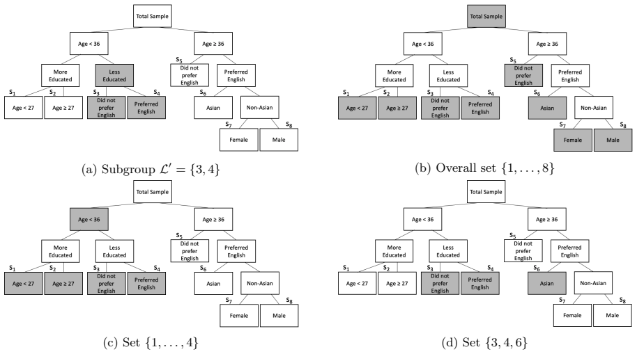
The load-bearing device is the absolute-difference construction: the tree is trained on $|Y_i|$, the absolute value of the adjusted outcome difference within each matched pair, rather than on the signed difference, so the instrument assignment $Z$ is hidden from the tree and the randomized assignment distribution inside matched pairs remains intact. This is combined with the matched-pair IV test statistic $T_s(\lambda_0)/S_s(\lambda_0)$ from the matching-IV literature and closed testing over all unions of the tree's leaves; the absolute difference makes every test level $\alpha$ under the sharp null, and closed testing converts level-$\alpha$ tests into strong familywise error control. The entity being tested is the H-CACE $\lambda_s = \frac{\sum_{i\in s}\sum_j (r^{(1)}_{1sij}-r^{(0)}_{0sij})}{\sum_{i\in s}\sum_j (d_{1sij}-d_{0sij})}$, which extends the usual complier average causal effect to a covariate-defined subgroup.
What would settle it
Simulate data with no true effect but with a rare covariate combination that forces the tree to create a leaf with very few pairs, run Algorithm 1 repeatedly, and compare the empirical familywise error rate to $\alpha$. If the small-leaf statistic is not approximately standard normal, the rejection rate will exceed $\alpha$, which would falsify Proposition 1 as an unconditional guarantee.
Extended reading notes
Core claim
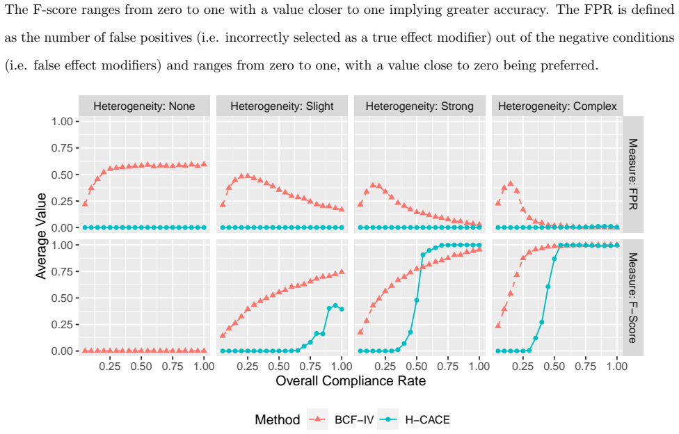
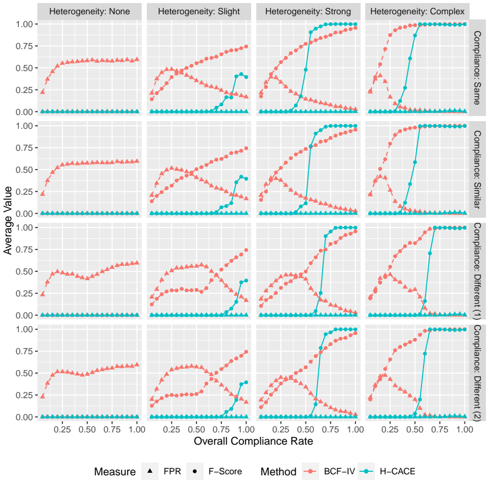
The paper's central result is Proposition 1: under the sharp null hypotheses used in Algorithm 1, the conditional probability, given the potential outcomes and covariates $F$, the instrument assignment $Z$, and the tree grouping $G$, that the algorithm makes at least one false rejection is at most $\alpha$. The mechanism is to feed the regression tree the absolute pairwise difference $|Y_i| = |(Z_{i1}-Z_{i2})(R_{i1}-\lambda_0 D_{i1} - (R_{i2}-\lambda_0 D_{i2}))|$ instead of the signed difference, so that the grouping depends only on $F$, not on $Z$; the instrument assignment therefore remains a fair coin within each matched pair, and the randomization-based null distribution used by the matching IV test statistics is preserved. The paper then runs closed testing over all unions of the tree's leaves, rejecting a subgroup hypothesis only when every superset hypothesis is rejected, which gives strong familywise error control. On the OHIE data the procedure reports significant H-CACEs in two subgroups, and simulations show high true discovery rates and low false-positive rates for effect modifiers, especially at low compliance rates.
Load-bearing premise
The guarantee rests on each subgroup test statistic $T_s(\lambda_0)/S_s(\lambda_0)$ being at least asymptotically level $\alpha$ under every sharp null visited by closed testing, even for the small, low-compliance leaves a regression tree can create, and on the tree being built from $X$ and $|Y|$ only so that the instrument assignment remains randomized within pairs.
Editorial extensions
If this is right
- Data-driven subgroup discovery and inference can be done on the full sample, so the method avoids the power loss of sample splitting while still controlling the familywise error rate.
- Any supervised grouping rule that uses only $X$ and $|Y|$ inherits the honesty property, so the same wrapper can be applied beyond the specific tree algorithm used here.
- In the paper's simulations, the method achieves high true discovery rates and near-zero false positive rates for effect modifiers even when compliance is below 40 percent, a regime where IV inference is usually weak.
- Subgroups with equal effect magnitudes but opposite signs are invisible to the method, because the absolute-value transformation collapses the direction of the effect.
- The OHIE analysis locates Medicaid's effect in older, English-preferring, non-Asian men and younger, English-preferring adults with at most a high school diploma or GED.
Reading between the lines
- Editorial inference: replacing the single tree with a forest would require each leaf's test to remain level $\alpha$, so an ensemble version would need either leaf-level calibration or a different multiplicity correction before the Proposition 1 guarantee could be claimed.
- Editorial inference: the closed-testing machinery is invertible in $\lambda_0$, so a natural extension would construct simultaneous confidence sets for all H-CACEs rather than testing a single fixed null value.
- Editorial inference: the OHIE tree depth was chosen by pruning back for interpretability, a judgment call that is not demonstrated to be independent of outcome-dependent information; an automatic, outcome-free tuning rule would make the procedure fully reproducible.
- Editorial inference: if the cited sharp-null-to-weak-null validity result holds generally, the procedure's error control would extend from sharp hypotheses to the weaker hypotheses $\lambda_s = \lambda_0$, which is what many users would care about in practice.
Signed reviews
Editorial analysis
A structured set of objections, weighed in public.
Referee Report
Summary. This paper proposes a method for discovering and testing heterogeneity in the complier average causal effect (H-CACE) in instrumental variables studies with paired matching. The method first pair-matches units on covariates, then grows a CART tree on the absolute value of the adjusted pairwise outcome difference |Y_i|, which is a function of the potential outcomes only under the sharp null, and finally applies closed testing to all unions of tree leaves using the IV test statistic of Baiocchi et al. (2010) and Kang et al. (2016). Proposition 1 claims strong familywise error control at level α conditional on (F, Z, G). The authors present simulations comparing the method with BCF-IV and apply it to the Oregon Health Insurance Experiment, reporting Medicaid effects among older English-preferring non-Asian men and younger English-preferring individuals with at most a high school diploma or GED.
Significance. The proposal addresses a real gap: existing tree-based heterogeneity methods for IV settings either rely on sample splitting or do not provide strong familywise error control, whereas the use of |Y| to decouple discovery from the instrument assignment is elegant and, if valid, permits honest inference without sample splitting. The H-CACE estimand is defined before estimation, so the analysis is not circular. The closed-testing structure is sound conditional on having level-α tests for every intersection hypothesis, and the OHIE application is a useful demonstration. However, the strength of the contribution depends on closing the gap between the imported asymptotic test and the sparse, data-dependent subsets used by CART, and on clarifying the tuning and matching assumptions.
major comments (4)
- [Web Appendix B; Eqs. (2)-(3); Algorithm 1] The proof of Proposition 1 in Web Appendix B reduces familywise error control to the claim that each intersection hypothesis H0L is tested at level α by |T_s(λ0)/S_s(λ0)|, and it states the equality P(|T/S| ≥ z_{1−α/2} | F,Z,G) = α/2. This equality is not exact in finite samples: the normal approximation is imported from Baiocchi et al. (2010) and Kang et al. (2016), where it is derived for a fixed matched sample with I growing, not for the variable, data-dependent unions of CART leaves that Algorithm 1 visits. In the OHIE analysis the nodes in Figure 4 have I_s in the hundreds and compliance near 0.29, so the subset statistics can have a much smaller effective sample of compliers; no uniform asymptotic or bounded-variance condition is provided for S_s(λ0). Please either prove the size property under explicit conditions on the class of possible groupings, or replace the normal approximation with an exact randomization test conditional on (F,Z,G), so that Proposition 1 holds exactly as stated.
- [Section 4.3; Algorithm 1, Step 3] Proposition 1 relies on G being a function of X and |Y| only. Section 4.3 reports that the OHIE tree depth was chosen by forming trees of larger depth and pruning back "until a more interpretable tree was obtained." If this search uses estimated subgroup effects, confidence intervals, or p-values, then G depends on Z and the conditional randomization argument fails. Please specify the exact tuning procedure for the complexity parameter, maximum depth, and pruning, and verify that it is a deterministic function of (X, |Y|) alone.
- [Section 2.3, Eqs. (4)-(5); Section 4.1] The definition of H-CACE at covariate value x is rewritten as a pair-subset estimand λ_s under the assumption that units within a matched pair have identical covariate values. The OHIE matching in Section 4.1 uses an optimal caliper and a robust rank-based Mahalanobis distance on age and several categorical variables, which does not generally yield exact covariate agreement within pairs. The paper does not define the pair-level covariate Xi used by CART or explain how approximate matching changes the interpretation of λ_s as a covariate-defined H-CACE. Please state the exact-matching assumption explicitly or redefine the estimand and the discovered subgroups at the level of matched pairs.
- [Web Appendix A, Table 1] The simulation evidence for finite-sample FWER is limited to one configuration with a strong signal (λ00=2, others 0), and the text itself notes that the trees from Y and |Y| are nearly identical at the upper levels in this configuration, so the simulation is not informative about the level of the subset-specific tests in the problematic small or low-compliance intersections. Please add simulations that report the size of |T_s(λ0)/S_s(λ0)| for sparse and low-compliance intersection hypotheses, or otherwise justify the asymptotic approximation in those settings.
minor comments (4)
- [Figures 1-2, 7-10] The simulation plots show averages over 1000 replications without Monte Carlo error bars or confidence bands; adding them would help interpret claims such as a false positive rate of zero.
- [Figure 9] The legend labels the comparison method as "BCV-IV"; this should read "BCF-IV."
- [Section 2.4] The statement that the honesty property is preserved for "any supervised machine learning algorithm" and "subsequent visual heuristics" is broader than what is proved; visual heuristics are not formal deterministic algorithms, and their independence from Z should be justified or the sentence qualified.
- [Web Appendix B] The proof writes "H0K : λs = λ0" for the subset null, but the algorithm's nulls are sharp unit-level nulls; aligning the notation would make the closed-testing argument easier to follow.
Circularity Check
No significant circularity: the FWER guarantee is a standard closed-testing argument, and the level-α test statistic is imported from independent prior work rather than fitted to this paper's data.
full rationale
The paper's central claim, Proposition 1, is proved in Web Appendix B by a conventional closed-testing reduction: under the sharp nulls, any false rejection of H0K requires rejection of the intersection H0T of all true hypotheses, and that intersection test is level α because |T(λ0)/S(λ0)| ≥ z_{1−α/2} has probability α/2 conditional on (F,Z,G). The paper does not fit any parameter and then rename it as a prediction; the H-CACE estimand is defined before estimation in Section 2.3, and the discovered subgroups are produced by CART on |Y|, which is a function of F only, preserving the randomization distribution of Z. The level-α property of the test statistic is cited from Baiocchi et al. (2010) and Kang et al. (2016), both published and externally established results that do not include the paper's target claim as an input; this is self-citation in the sense of shared authorship, but it is real, independent support rather than a circular reduction. The OHIE findings are outputs of the tree plus closed testing, not quantities forced by construction from the inputs. Concerns about the asymptotic approximation for sparse or low-compliance CART subsets are correctness or robustness issues, not circularity, and no specific equation in the paper reduces to an earlier fitted value or to the paper's own conclusion.
Assumptions & free parameters
free parameters (4)
- CART complexity parameter in OHIE analysis =
0
- CART maximum depth in OHIE analysis =
4
- CART complexity parameter in main simulations =
0.005
- OHIE-like simulation CART settings =
cp=0.001, max depth=7, min split=90
assumptions (4)
- domain assumption Instrumental variables assumptions (A1)-(A4): relevance, exclusion restriction, ignorability or exchangeability, and monotonicity.
- domain assumption Sharp null hypotheses H0L: r(d1)-r(d0)=lambda0(d1-d0) for all units in L.
- domain assumption Asymptotic standard normality of T_s(lambda0)/S_s(lambda0) under the sharp null.
- domain assumption The CART grouping G is a function of F only, not of the instrument assignment Z.
Cite this review
Pith. "Pith review of Detecting Heterogeneous Treatment Effect with Instrumental Variables." pith.science (2026). https://pith.science/paper/D27W3ITC
@misc{pith2026190803652,
  author       = {Pith},
  title        = {Pith review of: Detecting Heterogeneous Treatment Effect with Instrumental Variables},
  year         = {2026},
  howpublished = {\url{https://pith.science/paper/D27W3ITC}},
  note         = {Machine review of arXiv:1908.03652}
}
read the original abstract
There is an increasing interest in estimating heterogeneity in causal effects in randomized and observational studies. However, little research has been conducted to understand heterogeneity in an instrumental variables study. In this work, we present a method to estimate heterogeneous causal effects using an instrumental variable approach. The method has two parts. The first part uses subject-matter knowledge and interpretable machine learning techniques, such as classification and regression trees, to discover potential effect modifiers. The second part uses closed testing to test for the statistical significance of the effect modifiers while strongly controlling familywise error rate. We conducted this method on the Oregon Health Insurance Experiment, estimating the effect of Medicaid on the number of days an individual's health does not impede their usual activities, and found evidence of heterogeneity in older men who prefer English and don't self-identify as Asian and younger individuals who have at most a high school diploma or GED and prefer English.
Figures


Figures from the paper (8 more)





Reference graph
Works this paper leans on
-
[1]
Abadie, A. (2003). Semiparametric instrumental variable estimation of treatment response models. Journal of Econometrics , 113(2):231--263
2003
-
[2]
and Chen, X
Ai, C. and Chen, X. (2003). Efficient estimation of models with conditional moment restrictions containing unknown functions. Econometrica , 71(6):1795--1843
2003
-
[3]
D., Imbens, G
Angrist, J. D., Imbens, G. W., and Rubin, D. B. (1996). Identification of causal effects using instrumental variables. Journal of the American Statistical Association , 91(434):444--455
1996
-
[4]
and Imbens, G
Athey, S. and Imbens, G. (2016). Recursive partitioning for heterogeneous causal effects. Proceedings of the National Academy of Sciences , 113(27):7353--7360
2016
-
[5]
Recursive Partitioning for Heterogeneous Causal Effects
Athey, S. and Imbens, G. W. (2015). Machine learning methods for estimating heterogeneous causal effects. arXiv:1504.01132v1 [stat.ML]
work page Pith review arXiv 2015
-
[6]
Athey, S., Tibshirani, J., Wager, S., et al. (2019). Generalized random forests. The Annals of Statistics , 47(2):1148--1178
work page 2019
-
[7]
Baiocchi, M., Cheng, J., and Small, D. S. (2014). Instrumental variable methods for causal inference. Statistics in Medicine , 33(13):2297--2340
work page 2014
-
[8]
S., Lorch, S., and Rosenbaum, P
Baiocchi, M., Small, D. S., Lorch, S., and Rosenbaum, P. R. (2010). Building a stronger instrument in an observational study of perinatal care for premature infants. Journal of the American Statistical Association , 105(492):1285--1296
2010
Show all 55 references
-
[9]
and Pearl, J
Balke, A. and Pearl, J. (1997). Bounds on treatment effects from studies with imperfect compliance. Journal of the American Statistical Association , 92(439):1171--1176
1997
-
[10]
J., De-Witte, K., and Gnecco, G
Bargagli-Stoffi, F. J., De-Witte, K., and Gnecco, G. (2019). Heterogeneous causal effects with imperfect compliance: a novel bayesian machine learning approach. arXiv:1905.12707 [stat.ME]
2019 arXiv
-
[11]
Bargagli-Stoffi, F. J. and Gnecco, G. (2018). Estimating heterogeneous causal effects in the presence of irregular assignment mechanisms. In 2018 IEEE 5th International Conference on Data Science and Advanced Analytics (DSAA) , pages 1--10. IEEE
2018
-
[12]
Blundell, R., Chen, X., and Kristensen, D. (2007). Semi-nonparametric iv estimation of shape-invariant engel curves. Econometrica , 75(6):1613--1669
2007
-
[13]
and Powell, J
Blundell, R. and Powell, J. L. (2003). Endogeneity in nonparametric and semiparametric regression models. Econometric Society Monographs , 36:312--357
2003
-
[14]
Breiman, L., Friedman, J., Olshen, R., and Stone, C. (1984). Classification and Regression Trees. New York: Chapman and Hall/CRC
1984
-
[15]
and Pouzo, D
Chen, X. and Pouzo, D. (2012). Estimation of nonparametric conditional moment models with possibly nonsmooth generalized residuals. Econometrica , 80(1):277--321
2012
-
[16]
Chernozhukov, V., Demirer, M., Duflo, E., and Fernandez-Val, I. (2018). Generic machine learning inference on heterogenous treatment effects in randomized experiments. National Bureau of Economic Research
2018
-
[17]
Darolles, S., Fan, Y., Florens, J.-P., and Renault, E. (2011). Nonparametric instrumental regression. Econometrica , 79(5):1541--1565
2011
-
[18]
Ding, P. (2017). A paradox from randomization-based causal inference. Statistical Science , 32(3):331--345
2017
-
[19]
P., Allen, H., Baicker, K., and Group, O
Finkelstein, A., Taubman, S., Wright, B., Bernstein, M., Gruber, J., Newhouse, J. P., Allen, H., Baicker, K., and Group, O. H. S. (2012). The oregon health insurance experiment: evidence from the first year. The Quarterly Journal of Economics , 127(3):1057--1106
2012
-
[20]
Fogarty, C. B. (2018). Regression-assisted inference for the average treatment effect in paired experiments. Biometrika , 105(4):994--1000
2018
-
[21]
Fogarty, C. B. (2020). Studentized sensitivity analysis for the sample average treatment effect in paired observational studies. Journal of the American Statistical Association , 115(531):1518--1530
2020
-
[22]
B., Lee, K., Kelz, R
Fogarty, C. B., Lee, K., Kelz, R. R., and Keele, L. J. (2020). Biased encouragements and heterogeneous effects in an instrumental variable study of emergency general surgical outcomes. Journal of the American Statistical Association , pages 1--32
2020
-
[23]
R., Murray, J
Hahn, P. R., Murray, J. S., and Carvalho, C. (2017). Bayesian regression tree models for causal inference: regularization, confounding, and heterogeneous effects. arXiv:1706.09523 [stat,ME]
2017 arXiv
-
[24]
and Horowitz, J
Hall, P. and Horowitz, J. L. (2005). Nonparametric methods for inference in the presence of instrumental variables. The Annals of Statistics , 33(6):2904--2929
2005
-
[25]
Hern \'a n, M. A. and Robins, J. M. (2006). Instruments for causal inference: an epidemiologist's dream? Epidemiology , 17(4):360--372
2006
-
[26]
Hill, J. L. (2011). Bayesian nonparametric modeling for causal inference. Journal of Computational and Graphical Statistics , 20(1):217--240
2011
-
[27]
Hodges, J. L. and Lehmann, E. L. (1963). Estimates of location based on rank tests. The Annals of Mathematical Statistics , 34(2):598--611
1963
-
[28]
Y., Small, D
Hsu, J. Y., Small, D. S., and Rosenbaum, P. R. (2013). Effect modification and design sensitivity in observational studies. Journal of the American Statistical Association , 108(501):135--148
2013
-
[29]
Y., Zubizarreta, J
Hsu, J. Y., Zubizarreta, J. R., Small, D. S., and Rosenbaum, P. R. (2015). Strong control of the familywise error rate in observational studies that discover effect modification by exploratory methods. Biometrika , 102(4):767--782
2015
-
[30]
Imbens, G. W. (2010). Better late than nothing: Some comments on deaton (2009) and heckman and urzua (2009). Journal of Economic Literature , 48(2):399--423
2010
-
[31]
Kang, H., Kreuels, B., Adjei, O., Krumkamp, R., May, J., and Small, D. S. (2013). The causal effect of malaria on stunting: a mendelian randomization and matching approach. International Journal of Epidemiology , 42(5):1390--1398
2013
-
[32]
S., et al
Kang, H., Kreuels, B., May, J., Small, D. S., et al. (2016). Full matching approach to instrumental variables estimation with application to the effect of malaria on stunting. The Annals of Applied Statistics , 10(1):335--364
2016
-
[33]
Kang, H., Peck, L., and Keele, L. (2018). Inference for instrumental variables: a randomization inference approach. Journal of the Royal Statistical Society: Series A (Statistics in Society) , 181(4):1231--1254
2018
-
[34]
S., and Dominici, F
Lee, K., Small, D. S., and Dominici, F. (2018a). Discovering effect modification and randomization inference in air pollution studies. arXiv:1802.06710 [stat.AP]
2018 arXiv
-
[35]
S., Hsu, J
Lee, K., Small, D. S., Hsu, J. Y., Silber, J. H., and Rosenbaum, P. R. (2018b). Discovering effect modification in an observational study of surgical mortality at hospitals with superior nursing. Journal of the Royal Statistical Society: Series A (Statistics in Society) , 181(...
2018
-
[36]
S., and Rosenbaum, P
Lee, K., Small, D. S., and Rosenbaum, P. R. (2018c). A powerful approach to the study of moderate effect modification in observational studies. Biometrics , 74(4):1161--1170
2018
-
[37]
Marcus, R., Eric, P., and Gabriel, K. R. (1976). On closed testing procedures with special reference to ordered analysis of variance. Biometrika , 63(3):655--660
1976
-
[38]
Newey, W. K. and Powell, J. L. (2003). Instrumental variable estimation of nonparametric models. Econometrica , 71(5):1565--1578
2003
-
[39]
and Kang, H
Park, C. and Kang, H. (2020). A groupwise approach for inferring heterogeneous treatment effects in causal inference. arXiv preprint arXiv:1908.04427v2
2020 arXiv
-
[40]
Rosenbaum, P. R. (2002a). Covariance adjustment in randomized experiments and observational studies. Statistical Science , 17(3):286--327
2002
-
[41]
Rosenbaum, P. R. (2002b). [covariance adjustment in randomized experiments and observational studies]: Rejoinder. Statistical Science , 17(3):321--327
2002
-
[42]
Rosenbaum, P. R. (2010). Design of Observational Studies . New York: Springer
2010
-
[43]
Rosenbaum, P. R. (2020). Modern algorithms for matching in observational studies. Annual Review of Statistics and Its Application , 7:143--176
2020
-
[44]
Rubin, D. B. (1980). Randomization analysis of experimental data: The fisher randomization test comment. Journal of the American Statistical Association , 75(371):591--593
1980
-
[45]
Rubin, D. B. (2001). Using propensity scores to help design observational studies: application to the tobacco litigation. Health Services and Outcomes Research Methodology , 2(3-4):169--188
2001
-
[46]
Staiger, D. O. and Stock, J. H. (1997). Instrumental variables regression with weak instruments. Econometrica , 65(3):557--586
1997
-
[47]
H., Wright, J
Stock, J. H., Wright, J. H., and Yogo, M. (2002). A survey of weak instruments and weak identification in generalized method of moments. Journal of Business & Economic Statistics , 20(4):518--529
2002
-
[48]
Stuart, E. A. (2010). Matching methods for causal inference: A review and a look forward. Statistical Science , 25(1):1--21
2010
-
[49]
Su, L., Murtazashvili, I., and Ullah, A. (2013). Local linear gmm estimation of functional coefficient iv models with an application to estimating the rate of return to schooling. Journal of Business & Economic Statistics , 31(2):184--207
2013
-
[50]
M., and Li, B
Su, X., Tsai, C.-L., Wang, H., Nickerson, D. M., and Li, B. (2009). Subgroup analysis via recursive partitioning. Journal of Machine Learning Research , 10:141--158
2009
-
[51]
Swanson, S. A. and Hern \'a n, M. A. (2013). Commentary: how to report instrumental variable analyses (suggestions welcome). Epidemiology , 24(3):370--374
2013
-
[52]
Swanson, S. A. and Hern \'a n, M. A. (2014). Think globally, act globally: an epidemiologist’s perspective on instrumental variable estimation. Statistical Science , 29(3):371--374
2014
-
[53]
Therneau, T., Atkinson, B., and Ripley, B. (2015). Package ‘rpart’ . R package version 4.1-15. https://cran.r-project.org/package=rpart
2015
-
[54]
and Athey, S
Wager, S. and Athey, S. (2018). Estimation and inference of heterogeneous treatment effects using random forests. Journal of the American Statistical Association , 113(523):1228--1242
2018
-
[55]
Yu, R. (2019). bigmatch: Making Optimal Matching Size-Scalable Using Optimal Calipers . R package version 0.6.1. https://CRAN.R-project.org/package=bigmatch
2019
Reviewed August 14, 2026 · model on record in the stance chip above.
Discussion (0). Continue with ORCID to comment.