REVIEW 4 major objections 4 minor 24 references
Evolution of wind-generated shallow water waves in a Benney-Luke equation
T0 review · 4 major / 4 minor · reviewed 2026-08-07 · deepseek-v4-flash
Pith's one-line read This paper claims that adding wind forcing to the isotropic regularized Benney-Luke equation turns localized wave packets into two-dimensional solitary wave trains whose amplitudes grow or decay at rates set by the modulation equation (42).
desk verdict The new wind-forced BL model is worth a look, but the modulation theory's amplitude-width relation contradicts the paper's own traveling-wave equation, so the quantitative growth prediction is likely unsupported. read the letter →
The pith
A machine-rendered reading of the paper's core claim, the machinery that carries it, and where it could break.
The reading
What carries the argument
The load-bearing mechanism is the solitary-wave limit of wave modulation theory. A cnoidal wave of the BL equation has parameters $A,m,\Gamma,D,c,k,l$; as the elliptic modulus $m\to 1$ the wave becomes $\hat\zeta=A\,\mathrm{sech}^2(\gamma\theta)$ with $A=3\Gamma^2$, while $\kappa\to 0$ and $\Gamma=\gamma\kappa$ stays finite. Averaging the mass and energy conservation equations in this limit eliminates the mean-flow fields $D,F,G$ and leaves the single hyperbolic amplitude equation (42) for $\Gamma$, together with Hopf-type wavenumber equations (43). This reduction converts the full two-dimensional forced BL dynamics into a scalar growth law, equation (44), that the numerical experiments can test directly.
What would settle it
Extend the Figure 9 simulation beyond the finite-time blow-up $t=1/\alpha'$ of the modulation solution: the central claim fails if the tracked maximum of $\zeta$ does not first grow as $\Gamma_0^2/(1-\alpha' t)$ and then saturate or break near that time. A second check is to initialize the same case with small nonzero mean-flow fields $F,D,G$ in (35); if the growth rate changes by more than the $O(\epsilon)$ error, the zero-mean-flow assumption is the weak link.
Extended reading notes
Core claim
The central claim is that the wind-forced regularized Benney-Luke equation (12), derived here from the full Euler equations with $P_a=\alpha\zeta_x$, reproduces the solitary-wave-train phenomenology of the KdVB and KPB equations despite being isotropic in the horizontal plane. The paper shows that its cnoidal waves have the same structure as KdV cnoidal waves, and that in the $m\to 1$ solitary-wave limit the averaged mass and energy equations reduce to the single modulation equation for $\Gamma$, equation (42). Solving that equation with time-only dependence gives $\Gamma^2=\Gamma_0^2/(1-\alpha' t)$ with $\alpha'=\alpha(k/\kappa)(32\Gamma_0^2/45)$, predicting finite-time amplitude blow-up for positive forcing and decay for negative forcing. Long-time pseudospectral simulations in narrow domains form solitary wave trains, and the tracked maximum of $\zeta$ follows the predicted growth curve (Figure 9). In wide domains, isotropic $y$-dispersion bends wave fronts into circular arcs and can prevent train formation, a qualitative difference from the anisotropic KP model.
Load-bearing premise
The load-bearing premise is that the emerging wave train can be described as a slowly varying solitary wave on a zero mean flow, so the amplitude parameter $\Gamma$ alone controls the growth; if the neglected mean flow or finite-wavenumber corrections feed back into the amplitude evolution, the predicted rate (44) used in Figure 9 would not match the full Benney-Luke dynamics.
Editorial extensions
If this is right
- In narrow domains, small initial wavenumbers and large initial amplitudes are the favorable conditions for solitary wave train formation; the paper's simulations show trains emerging near $x=600$–$700$ by $t=1000$.
- With $\beta'>0$ the downstream solitary waves and the upstream radiation both grow, and the downstream amplitude follows $\Gamma^2=\Gamma_0^2/(1-\alpha' t)$, while $\beta'<0$ gives decay on the $|\alpha'|^{-1}$ time scale.
- Wide-domain initial conditions generate circular wave fronts because the BL equation is isotropic, and this two-dimensional dispersion delays or prevents solitary wave formation.
- As $\epsilon\to 0$ the BL equation reduces asymptotically to the KPB equation, so the KPB solitary-wave results are recovered as a special case of the present model.
Reading between the lines
- Editorial inference: because the modulation reduction discards the mean flow before comparing with numerics, the same method should apply to any isotropic Boussinesq-type equation with a Burgers-type forcing term; the growth law (44) may be generic for weakly nonlinear, weakly dispersive two-dimensional shallow-water systems.
- Editorial inference: the isotropic geometry implies that oblique wave trains with nonzero $l_0$ should grow along the ray direction $(k/\kappa,l/\kappa)$ rather than only downstream, so soliton-gas statistics in this model are not locked to the wind axis.
- Editorial inference: a direct test of the soliton-gas claim would be to count resolved solitary pulses in the narrow-domain simulations over time and compare the pulse-number density with the amplitude growth law, which the paper does not do.
Editorial analysis
A structured set of objections, weighed in public.
Referee Report
Summary. The paper derives a wind-forced, regularized Benney-Luke (BL) equation as an isotropic two-dimensional model for shallow-water waves, studies its cnoidal and solitary-wave solutions, develops a modulation theory for solitary wave trains, and presents numerical simulations showing the emergence of solitary-wave trains from localized initial conditions. The central quantitative claim is that the amplitude Γ of the solitary wave train obeys the modulation equation Γ_t + (k/κ)Γ_x + (l/κ)Γ_y = α(k/κ)(16Γ³/45), whose t-only solution (44) predicts the growth rate that is compared with numerics in Fig. 9(b).
Significance. If the modulation-theoretic prediction were correct, this would be a valuable extension of the authors' earlier KdVB and KPB soliton-gas studies to an isotropic, two-way BL model, with possible relevance to shallow-water wind-wave forecasting. The paper contains extensive numerical experiments, a clearly described pseudospectral scheme, and a genuine external comparison (Fig. 9) that is not fitted to the data. However, the quantitative modulation theory is not reliable as written: the amplitude–width relation used to derive it is inconsistent with the stated travelling-wave ODE, and the energy-source expression appears to contain an algebraic error. The qualitative observation of solitary-wave-train formation is interesting, but the central quantitative claim needs substantial correction and verification.
major comments (4)
- [§3.1, Eqs. (28)–(30), (34)] The amplitude–width relation A = 3mΓ² stated in (30) and used in the solitary-wave limit (34) does not satisfy the travelling-wave ODE (28). Substituting ζhat = A sech²(γθ) with Γ = κγ into (28) and equating the sech⁴ coefficients gives -2AΓ² + (3/2)κA² = 0, hence A = 4Γ²/(3κ), not A = 3Γ²; with κ → 0 at fixed Γ the amplitude diverges, so the m → 1 limit taken in §3.3 is not a solitary-wave limit of (28). Since E and F in (41), the modulation equation (42), and the growth law (44) all use A = 3Γ², this is a load-bearing inconsistency. If (28) contains a typographical error in the coefficient of the nonlinear term, that error must be corrected and the averaging calculation shown.
- [§3.2, Eqs. (36)–(41)] Independent of the amplitude–width issue, the energy-source expression appears to have an algebraic error. For ζhat = A sech²(γθ) a direct average gives <ζθ²> = 8A²γ/(15π), so J = ωk<ζθ²> = 8kA²Γ/(15π). In the m → 1 limit, (38) with C4 − C6 = 2/(15πγ) gives J = (k/κ)(16/3)A²Γ²(C4 − C6) = 32kA²Γ/(45π), a factor 4/3 larger. The subsequent \bar F in (41), the coefficient 16/45 in (42), and α′ in (44) inherit this factor. The averaging steps leading to (37)–(41) should be presented in full.
- [§3.2–3.3, Eqs. (35), (42)] The modulation equations are derived after setting D = 0, F = 0, G = 0 in (35) without an estimate of the mean-flow feedback. Equation (35) shows that D evolves in response to E, and the paper itself notes that D varies oppositely to E; for a solitary wave train generated from a localized initial condition this mean flow is not obviously negligible on the time scale of (44). The authors should provide an order-of-magnitude estimate of the D, F, G contributions to (42), or demonstrate numerically that including them does not change the predicted growth rate.
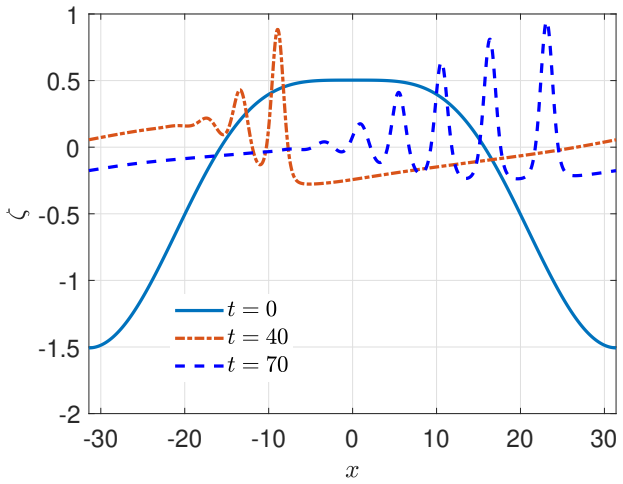
- [§4, Fig. 9] The quantitative check in Fig. 9(b) does not state how Γ0 is extracted from the initial condition or from the numerically tracked maximum, and the comparison uses the t-only solution (44) even though the simulated wave train is spatially inhomogeneous (the maximum is sought over x > 300). Given the issues above, the reported 'good agreement' cannot be regarded as a validated prediction of the BL equation until the modulation theory is corrected and the comparison protocol is specified.
minor comments (4)
- [§3.3, Eq. (52)] Equation (52) appears to be incomplete: the right-hand side reads '=,' and should presumably be '= 0'.
- [§2 and §3.2] The symbol F is used both for the horizontal energy flux in (20) and for the source term in (38)–(41); this overloading is confusing and should be distinguished.
- [§4, Fig. 9] The caption of Fig. 9(b) says 'predicted growth and decay rates when β′ = ±0.001', but the text only describes the case β′ = 0.001; the decay case should be shown or the caption adjusted.
- [References] The comparison with Maleewong and Grimshaw (2025) is central, but that reference is listed as 'Submitted'; if possible, a published or arXiv version should be cited.
Circularity Check
No significant circularity: the modulation-theory growth law (44) is derived from the averaged BL energy equation and compared with numerical maxima using a prescribed forcing coefficient, not fitted to the target curve.
full rationale
The paper's central quantitative prediction is the solitary-wave amplitude growth law (44), obtained by substituting the solitary-wave energy and flux expressions (41) into the modulation energy equation (40). This is an algebraic derivation from the averaged conservation equations, not a fit to the numerical maximum shown in Fig. 9(b). The forcing parameter β′ is prescribed (Table 1, Fig. 9) and Γ0 in (44) is the initial value of the modulation variable, not a parameter inferred from the comparison data. The numerical simulations solve the full BL system (14)/(59) independently of the modulation reduction, so agreement with (44) is a genuine check. Self-citations to Maleewong and Grimshaw (2024b, 2025) supply the KdVB/KPB methodology and a comparison of qualitative behavior, but the BL modulation equations are derived in Sections 3.2–3.3 from the BL system itself, and the traveling-wave/cnoidal solutions are attributed to Benney and Luke (1964) and Ablowitz and Curtis (2011), not to a self-citation. No fitted parameter is renamed as a prediction, and no uniqueness theorem or ansatz is imported solely from the authors' prior work. Any concern about the formal consistency of the amplitude–width relation A = 3Γ² with the travelling-wave ODE (28) is a correctness/validity issue, not a circularity issue, since the numerical check does not enforce that relation by construction.
Assumptions & free parameters
free parameters (3)
- Wind forcing coefficient β′ (or α) =
0, 0.001 (and sign varied)
- Initial condition parameters (A, k0, l0, LX, LY) =
Varies per case, e.g., A=0.5, k0=1.27, l0=0.1, LX=LY=30
- Numerical domain and sponge parameters (PX, PY, ν, κs, wd) =
e.g., PX=400π/k0, PY=10π, ν=1, κs=0.4, wd=1.85
assumptions (5)
- domain assumption The fluid is inviscid, incompressible, of constant density, with irrotational flow and a rigid horizontal bottom.
- domain assumption The long-wave asymptotic balance β=ǫ (amplitude and dispersion parameters equal) is assumed so that nonlinearity and dispersion are comparable.
- domain assumption Wind forcing is modelled by surface pressure Pa = α ζ_x with constant α, based on Miles critical-layer theory.
- domain assumption The BL equation is regularized to avoid spurious high-wavenumber instability, changing the dispersion relation at large wavenumbers.
- ad hoc to paper Wave modulation theory assumes a slowly varying periodic wave and neglects the mean flow by setting D=0, F=0, G=0.
Cite this review
Pith. "Pith review of Evolution of wind-generated shallow water waves in a Benney-Luke equation." pith.science (2026). https://pith.science/paper/D4PWEOVD
@misc{pith2026250600399,
  author       = {Pith},
  title        = {Pith review of: Evolution of wind-generated shallow water waves in a Benney-Luke equation},
  year         = {2026},
  howpublished = {\url{https://pith.science/paper/D4PWEOVD}},
  note         = {Machine review of arXiv:2506.00399}
}
read the original abstract
In recent papers, denoted by MG24, MG25 in this text, we used the Korteweg-de Vries (KdV) equation and its two-dimensional extension, the Kadomtsev-Petviashvili (KP) equation to describe the evolution of wind-driven water wave packets in shallow water. Both equations were modified to include the effect of wind forcing, modelled using the Miles critical level instability theory. In this paper that is extended to a Benney-Luke (BL) equation, similarly modified for wind forcing. The motivation is that the BL equation is isotropic in the horizontal space variables, unlike the KP model, and noting that the KdV model is one-dimensional. The modified BL equation is studied using wave modulation theory as in MG24, MG25, and with comprehensive numerical simulations. Despite the very different spatial structure the results show that under the right initial conditions and parameter settings, solitary wave trains emerge as in MG24, MG25.
Figures


Figures from the paper (6 more)


Reference graph
Works this paper leans on
-
[1]
Ablowitz, M. J. and Curtis, C. W. (2011). On the evolution of perturbations to solutions of the K adomtsev P etviashvilli equation using the B enney- L uke equation. J. Phys. A: Math. Theor. , 44:195202
work page 2011
-
[2]
Ablowitz, M. J. and Curtis, C. W. (2013). Conservation laws and non-decaying solutions for the B enney- L uke equation. Proc. Royal Soc. A , 469:20120690
work page 2013
-
[3]
Benney, D. J. and Luke, J. C. (1964). On the interactions of permanent waves of finite amplitude. Journal of Mathematics and Physics , 43:309--313
work page 1964
-
[4]
Costa, A., Osborne, A. R., Resio, D. T., Alessio, S., isabetta Chriv, Saggese, E., Bellomo, K., and Long, C. E. (2014). Soliton turbulence in shallow water ocean surface waves. Phys. Rev. Lett. , 113:108501
work page 2014
-
[5]
El, G., Hoefer, M. A., and Shearer, M. (2016). Expansion shock waves in regularized shallow water theory. Proc. Roy. Soc. A , 472:20160147
work page 2016
-
[6]
El, G. A. (2021). Soliton gas in integrable dispersive hydrodynamics. J. Stat. Mech. , --:114001
work page 2021
-
[7]
Fornberg, B. and Whitham, G. B. (1978). A numerical and theoretical study of certain nonlinear wave phenomena. Phil.Trans. Royal Soc. A , 289:373--404
work page 1978
-
[8]
Grava, T., Klein, C., and Pittori, G. (2018). Numerical study of the K adomtsev- P etviashvili equation and dispersive shock waves. Proc. Royal Soc. A , 474:20170458
work page 2018
Show all 24 references
-
[9]
Grimshaw, R., Hunt, J., and Johnson, E. (2018). I U T A M S ymposium W ind W aves, 2017 , volume 26. Elsevier IUTAM Procedia Series
2018
-
[10]
and Yuan, C
Grimshaw, R. and Yuan, C. (2016). The propagation of internal undular bores over variable topography. Physica D , 333:200--207
2016
-
[11]
Janssen, P. (2004). The interaction of ocean waves and wind . Cambridge University Press, UK
2004
-
[12]
A., Manna, M
Kharif, C., Kraenkel, R. A., Manna, M. A., and Thomas, R. (2010). The modulational instability in deep water under the action of wind and dissipation. J. Fluid Mech. , 664:138--149
2010
-
[13]
and Roidot, K
Klein, C. and Roidot, K. (2011). Fourth order time-stepping for K adomtsev- P etviashvili and D avey- S tewartson equations. SIAM J. Sci Comput. , 33:3533--3556
2011
-
[14]
and Grimshaw, R
Maleewong, M. and Grimshaw, R. (2024a). Evolution of water wave groups in water of finite depth. J. Fluid Mech. , 985:A2
2024
-
[15]
and Grimshaw, R
Maleewong, M. and Grimshaw, R. (2024b). Evolution of water wave packets by wind in shallow water. J. Fluid Mech. , 996:A4
2024
-
[16]
and Grimshaw, R
Maleewong, M. and Grimshaw, R. (2025). Evolution of wind-generated shallow water waves in the framework of a modified K adomtsev- P etviashvili equation. Fluids , Submitted:--
2025
-
[17]
Manna, M. A. and Latifi, A. (2023). Korteweg-de V ries- B urger equation with J effreys wind wave interaction: blow-up and breaking of soliton-like solutions in finite time. Fluids , 8:231--244
2023
-
[18]
Miles, J. W. (1957). On the generation of surface waves by shear flows. J. Fluid Mech. , 3:185--204
1957
-
[19]
Milewski, P. A. and Tabak, E. (1999). A pseudospectral procedure for the solution of nonlinear wave equations with examples from free-surface flows. SIAM J. Sci. Comput. , 21:1102--1114
1999
-
[20]
R., Jannsen, P
Onorato, M., Osborne, A. R., Jannsen, P. A. E. M., and Resio, D. (2009). Four-wave resonant interactions in the classical quadratic B oussinesq equations. J. Fluid Mech. , 618:263--277
2009
-
[21]
Osborne, A. R. (2010). Nonlinear ocean waves and the inverse scattering transform . Elseveier
2010
-
[22]
Whitham, G. B. (1974). Linear and N onlinear W aves. Wiley
1974
-
[23]
Zabusky, N. J. and Kruskal, M. D. (1965). Interaction of solitons in a collisionless plasma and the recurrence of initial states. Phys. Rev. Letters , 15:240--243
1965
-
[24]
and Feddersen, F
Zdyrski, T. and Feddersen, F. (2021). Wind-induced changes to surface gravity wave shape in shallow water. J. Fluid Mech. , 903:A27
2021
Reviewed August 7, 2026 · model on record in the stance chip above.
Discussion (0). Sign in to comment.