REVIEW 2 major objections 5 minor 2 cited by
Quantum computational sensing using quantum signal processing, quantum neural networks, and Hamiltonian engineering
T0 review · 2 major / 5 minor · reviewed 2026-08-06 · deepseek-v4-flash
Pith's one-line read Interleaving sensing with quantum computation before measurement classifies signals more accurately than estimating them first, with simulated gains over 20 percentage points at equal sensing time.
desk verdict A coherent framework with clean bosonic analytics, but the headline static-signal advantage is an artifact of a baseline that forbids coherent integration; worth refereeing with that fixed. read the letter →
The pith
A machine-rendered reading of the paper's core claim, the machinery that carries it, and where it could break.
The reading
What carries the argument
The load-bearing object is the interleaved circuit $U_{\rm QCS}=U_{\rm meas}\prod_{l=1}^{L}U_{\rm sense}(u^{(l)})U_{\rm coh}^{(l)}$: $L$ signal-dependent sensing operations alternating with $L$ coherent computing operations before a single measurement. Because the signal enters several times, the circuit can realize nonlinear functions of it: for a single qubit, quantum-signal-processing rotations (the QSP construction in which interleaved non-commuting rotations implement polynomial functions of an input phase); for several qubits, trainable unitaries of the kind used in quantum neural networks; for bosonic modes, a nonlinear quantum non-demolition amplifier $\hat{H}_{\rm NL}=\sqrt{2}g\,\hat{f}\hat{P}_b$ with Hermitian $\hat{f}=\sum Q_{nm}\hat{a}^{\dagger n}\hat{a}^m$, whose readout-mode heterodyne outcome has mean $g\langle\hat{f}\rangle$ and therefore directly outputs the desired polynomial of the sensed displacement. The same design principle appears in every platform: target functions are engineered so that measurement probabilities saturate toward 0 or 1, and because single-qubit sampling variance vanishes at those extremes, this both performs the classification and suppresses the quantum sampling noise that limits the conventional baseline — the property that makes single-shot operation work.
What would settle it
For a static phase signal, compute the classification error of a single Ramsey measurement that coherently integrates over the full $N$ periods (one shot of duration $N\cdot\tau$) and compare it with the QCS error at the same $N$ for the single-qubit task of Fig. 2. If the long coherent Ramsey baseline reaches or beats the QCS error, the claimed quantum computational advantage for static single-qubit classification does not survive a matched-coherence comparison; if QCS still wins, the advantage is genuinely nonlinear processing rather than coherence accounting.
Extended reading notes
Core claim
The central claim is that coherently processing a signal inside the sensor before measurement can beat the standard strategy of estimating the signal and then deciding classically, whenever the task is to compute a nonlinear function of the signal. The architecture is the unitary $U_{\rm QCS}=U_{\rm meas}\prod_{l=1}^{L}U_{\rm sense}(u^{(l)})U_{\rm coh}^{(l)}$, in which $L$ sensing operations are interleaved with $L$ trainable computing operations before one measurement; for qubit sensors the computing layers are quantum-signal-processing rotations (single qubit) or trainable multi-qubit unitaries (quantum-neural-network style), while for bosonic sensors the computation is done by a nonlinear quantum non-demolition amplifier with Hamiltonian $\hat{H}_{\rm NL}=\sqrt{2}g\,\hat{f}\hat{P}_b$, where choosing $\hat{f}=\sum_{n,m}Q_{nm}\hat{a}^{\dagger n}\hat{a}^m$ makes a heterodyne readout directly return a chosen polynomial of the displacement $\alpha$. All protocols are compared with conventional quantum-sensing baselines at equal total sensing periods $N$, and for every task the paper reports a regime in which the quantum computational sensor reaches lower classification error or lower mean-squared error, with the gap growing as the task becomes harder.
Load-bearing premise
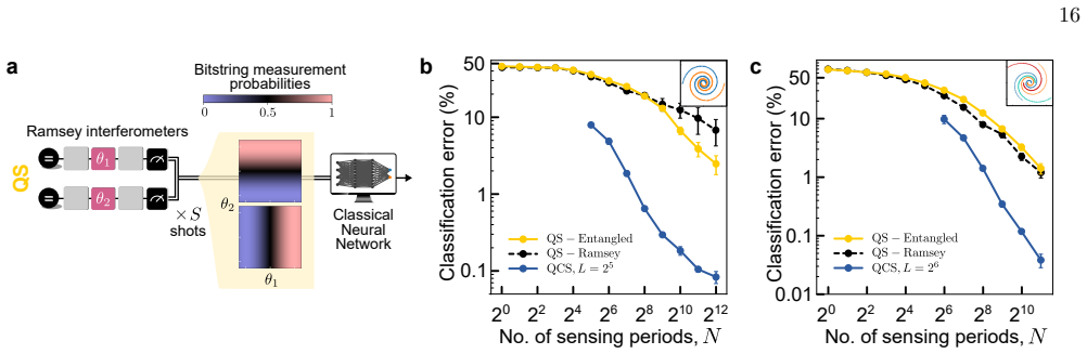
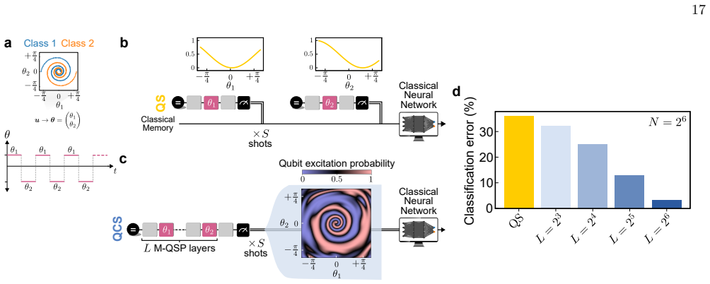
The conventional sensor is benchmarked as many separate one-period measurements, while the quantum computational sensor uses all $N$ sensing periods in one unbroken run; the paper does not compare against a conventional sensor that also integrates the whole signal coherently, so part of the reported advantage may come from that asymmetry.
Editorial extensions
If this is right
- For a fixed budget of $N$ sensing periods, a protocol with $L$ interleaved computing layers reaches lower classification error than the conventional sensor at the same $N$, and the largest advantage occurs in the single-shot limit $L=N$, $S=1$.
- The advantage grows with task complexity: for single-variable tasks with $R$ noncontiguous class regions, the conventional sensor's error scales approximately as $0.063(2R-1)$ while the QCS error scales approximately as $0.015(2R-1)$ at $N=64$, so harder tasks show larger gaps.
- A single qubit suffices for binary classification, $M=\log_2 C$ qubits suffice for single-shot $C$-class discrimination, and a one-qubit-plus-one-bosonic-mode hybrid sensor classifies the Circles task at 1.7% error versus 11.2% for the conventional protocol.
- A bosonic sensor with an engineered nonlinear amplifier estimates arbitrary polynomials of a complex displacement with lower variance than a phase-preserving linear amplifier followed by classical postprocessing; for the XOR task the QCS estimator variance is half the QS variance at large gain.
- Training can be done end-to-end on finitely sampled measurement results — even a single shot per inference — so the protocols do not require exact outcome probabilities or expectation values.
Reading between the lines
- A direct test the paper does not run: for static signals, compare against a single Ramsey measurement that coherently integrates over the full $N$ periods. If that baseline matches the QCS error, part of the reported advantage is coherence accounting rather than nonlinear processing; if QCS still wins, the advantage is genuine computation in the sensor.
- The resource relation $N = L \times S$ implies a measurable tradeoff curve: for fixed $N$, classification error plotted against $L$ should dip to a minimum whose position shifts with task complexity, a signature a small experimental device could check in a few parameter sweeps.
- The design principle of pushing final measurement probabilities toward 0 and 1 to suppress sampling noise is task-agnostic and may transfer beyond sensing to any few-shot quantum classifier trained on noisy hardware.
Editorial analysis
A structured set of objections, weighed in public.
Referee Report
Summary. The paper proposes a general framework for quantum computational sensing (QCS) in which L sensing operations are interleaved with L coherent processing operations before a single measurement, and applies it to qubit-based, bosonic, and hybrid qubit-bosonic platforms. The tasks include binary and multiclass classification of static phases, classification of time-varying spatiotemporal MEG signals, and polynomial function approximation of complex displacements. The authors compare each QCS protocol against a conventional quantum sensing (QS) baseline that first estimates the signal and then classically postprocesses, reporting accuracy advantages that in several simulated tasks exceed 20 percentage points at equal total sensing periods N. Training is performed with finitely sampled measurement outcomes, including single-shot inference, and the bosonic protocols are supported by analytic derivations of unbiased estimators and their variances.
Significance. If the comparative claims are upheld, the paper would be a substantial contribution to quantum sensing: it unifies several QCS proposals under one architecture, demonstrates finite-shot training with single-shot inference, and provides clean analytic constructions for bosonic function approximation. The availability of code and data is a strength, as is the explicit treatment of sampling noise in the training objective. However, the headline claim of a sensing-time advantage currently rests on a conventional-sensor baseline that is restricted in a way that may unfairly favor the QCS protocols, and the MEG results involve a post-selection procedure that is not fully specified. These issues need to be resolved before the central claim can be accepted.
major comments (2)
- [Sec. III A, Appendix B 5, Figs. 2f, 3e, 3k]
- [Appendix C 4, Appendix C 5, Fig. 17]
minor comments (5)
- [Sec. III A]
- [Fig. 2f inset]
- [Appendix C 4]
- [Sec. III D]
- [Sec. IV D]
Circularity Check
No significant circularity: the paper's analytic constructions and numerical claims are self-contained; the main caveat is a benchmark-fairness question, not a circular reduction.
full rationale
All load-bearing derivations are carried out within the paper. For the qubit QSP/QNN protocols (Sec. III A-C and App. B), the QCS circuits are trained on finite-shot samples with a separate test evaluation; the reported errors are Bayes/MLP test errors, not re-statements of the training loss. The analytic QS error expression in App. B 5 is derived from a Gaussian approximation to binomial Ramsey statistics and is then compared with independently trained QCS errors; it does not assume the QCS result. For bosonic function approximation (Sec. IV and App. D), the QCS estimator FQCS = (1/2g)(X + X*) with f = sum Wnm a†^n a^m gives E[FQCS] = F* by explicit construction, and the QS coefficients Cnm are likewise solved from the unbiasedness condition; the MSE comparison is a variance computation, not an equivalence. The hybrid sensor protocol (Sec. V) is trained with a fixed resource constraint (equal average photon number) and evaluated on held-out test data. The only self-citation with overlapping authors is the companion QCSA paper [1], used to introduce terminology and prior context; none of the paper's quantitative advantage claims depend on it. A legitimate benchmark-fairness caveat exists: the conventional QS baseline is taken as S = N independent single-period Ramsey shots (Sec. III A, Fig. 2f; Sec. III C, Figs. 3e and 3k), while QCS uses all N periods coherently in a single shot; the paper does not benchmark against a conventional Ramsey sensor that coherently integrates for the full N periods. That is a potential overstatement of the reported advantage, but it is a modeling/comparison choice rather than a circular reduction of a prediction to its inputs.
Assumptions & free parameters
free parameters (5)
- trainable QCS circuit angles and unitaries =
learned per task
- Qnm coefficients for bosonic nonlinear amplifier =
Spirals coefficients in Table VI; XOR: ±i
- hybrid ansatz parameters β^(d), R^(d) =
learned, D=16 layers
- MEG signal scaling / RMS phase θ_RMS =
varied 0.0 to 0.3
- hyperparameters L, S, T =
L up to 2^6, T=10, S=1
assumptions (5)
- domain assumption Quantum mechanics: unitary evolution and projective measurement, with ideal noiseless operation.
- standard math QSP/QNN expressivity: L interleaved sensing operations can realize polynomial functions of the sensed parameter.
- domain assumption Nonlinear amplifier solution b_out = b_in + g f for the QND Hamiltonian H_NL = -ig f(b - b†).
- domain assumption The MEG dataset is treated as a 'quantum noise-free' ground truth, scalable to arbitrary RMS phase.
- domain assumption Training uses exact gradients of the quantum circuit (analytic backpropagation) although the forward loss is evaluated on finite samples.
Cite this review
Pith. "Pith review of Quantum computational sensing using quantum signal processing, quantum neural networks, and Hamiltonian engineering." pith.science (2026). https://pith.science/paper/D74GTFJO
@misc{pith2026250715845,
  author       = {Pith},
  title        = {Pith review of: Quantum computational sensing using quantum signal processing, quantum neural networks, and Hamiltonian engineering},
  year         = {2026},
  howpublished = {\url{https://pith.science/paper/D74GTFJO}},
  note         = {Machine review of arXiv:2507.15845}
}
abstract
Combining quantum sensing with quantum computing can lead to quantum computational sensors that are able to more efficiently extract task-specific information from physical signals than is possible otherwise. Early examples of quantum computational sensing (QCS) have largely focused on protocols where only a single sensing operation appears before measurement -- with an exception being the recent application of Grover's algorithm to signal detection. In this paper we present, in theory and numerical simulations, the application of two quantum algorithms -- quantum signal processing and quantum neural networks -- to various binary and multiclass machine-learning classification tasks in sensing. Here sensing operations are interleaved with computing operations, giving rise to nonlinear functions of the sensed signals. We have evaluated tasks based on static and time-varying signals, including spatiotemporal signals. Our approach to optimizing the circuit parameters in a QCS protocol takes into account quantum sampling noise and allows us to engineer protocols that can yield accurate results with as few as just a single measurement shot. In all cases, we have been able to show a regime of operation where a quantum computational sensor can achieve higher accuracy than a conventional quantum sensor, with a simulated accuracy advantage of $>$20 percentage points for some tasks. We also present protocols for performing nonlinear tasks using Hamiltonian-engineered bosonic systems and quantum signal processing with hybrid qubit-bosonic systems. Overall, we have shown that substantial quantum computational-sensing advantages can be obtained even if the quantum system is small, including few-qubit systems, systems comprising a single qubit and a single bosonic mode, and even just a single qubit alone -- raising the prospects for experimental proof-of-principle and practical realizations.
Figures


Figures from the paper (19 more)




Forward citations
Cited by 2 Pith papers
-
Simple broadband signal detection at the fundamental limit
Broadband AC-field detection at the Grover-like limit can be achieved by a single analog experiment using a randomized SSH control Hamiltonian and a GHZ probe, with the lower bound derived from an integrated-quantum-F...
-
Quantum Computational-Sensing Advantage
A perspective defines quantum computational sensing (QCS) and its advantage (QCSA), and organizes many recent sensing-plus-computing protocols into a single taxonomy.
Reference graph
Works this paper leans on
-
[1]
Dataset and classification task The dataset we use for these simulations is obtained from an open-source experiment [21]. The dataset is a time- varying, 306-channel magnetoencephalography (MEG) signal, along with a 3-axis accelerometer signals. Each channel consists of data generated by a sensor. There are 3 sensors at 102 spatial locations on a headset....
-
[2]
Dataset preprocessing We now discuss the procedure we implement to allow the dataset to be compatible with our simulations. The main goal of this procedure is to reduce the complexity of the simulation of the quantum system, so that they maybe simulated in a reasonable time on a classical computer. We first perform Principal Component Analysis on the data...
-
[3]
% 1 M · T T emporally-coherent QCS (T)
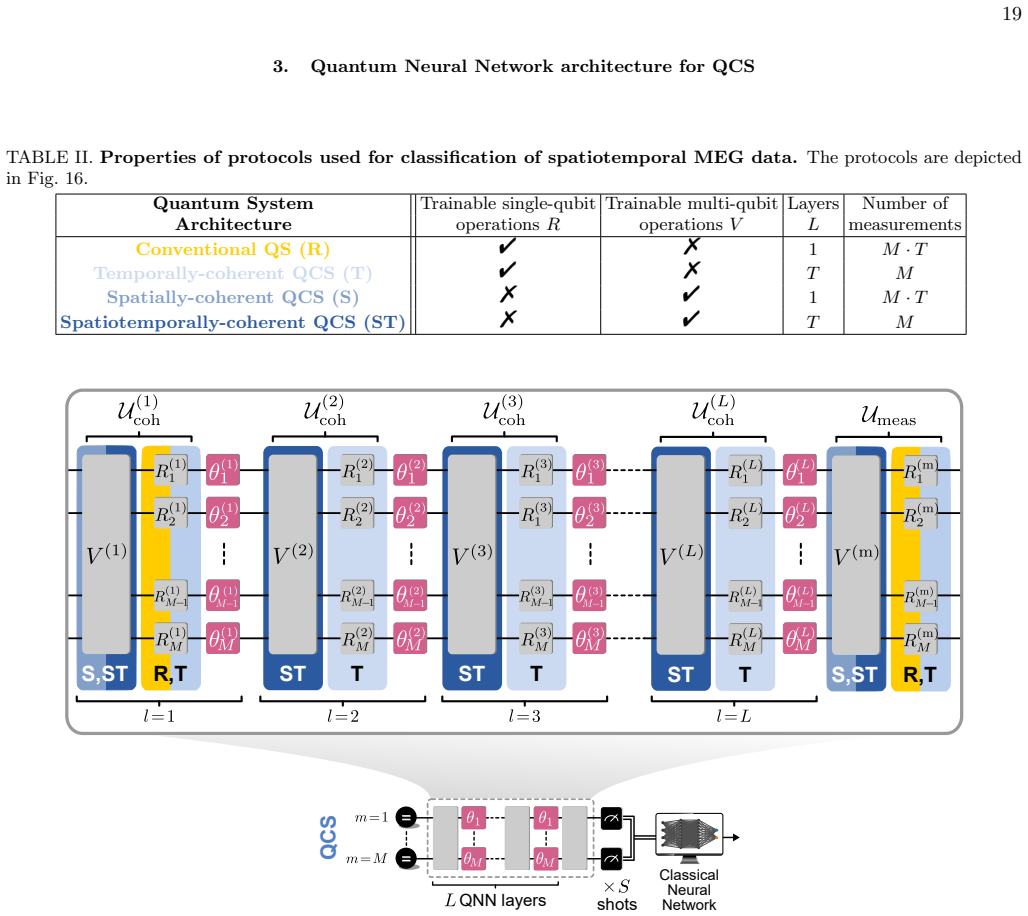
Quantum Neural Network architecture for QCS TABLE II. Properties of protocols used for classification of spatiotemporal MEG data. The protocols are depicted in Fig. 16. Quantum System Trainable single-qubit Trainable multi-qubit Layers Number of Architecture operations R operations V L measurements Conventional QS (R) " % 1 M · T T emporally-coherent QCS ...
-
[4]
T raining details The simulations are performed with PyTorch [37], which allows us to use the conventional method of backpropa- gation to train the system. All matrices, representing the sensing and programmable unitaries, and the state of the system, are stored as PyTorch tensors (with a dimension set by the Hilbert space size of the system), allowing fo...
work page 2000
-
[5]
Additional results Ramsey interferometry Temporally-coherent Spatially-coherent Spatiotemporally-coherent 0.0 0.1 0.2 0.3 Ramsey interferometry Temporally-coherent Spatially-coherent Spatiotemporally-coherent 40 30 20 0.0 0.1 0.2 0.3 50Classification error (%) Signal strength (average imparted phase ) Ramsey interferometry Temporally-coherent Spatially-co...
-
[6]
QCSA vs. task complexity for more general tasks To emphasize that the performance difference between QS and QCS protocols for increasing task difficulty is not special to the tasks considered in Appendix B 5, we now compare their performance for more general tasks. In particular, while we still consider our general binary classification tasks with R nonco...
-
[7]
Multi-variate sensing: comparing quantum computational sensors against multiple Ramsey interferometers In Sec. III C of the main text, for the conventional QS benchmark we consider a protocol for which Uprobe and Umeas are entangling operations and L = 0, namely with a structure similar to quantum sensor networks [2]. In particular, this quantum sensor is...
-
[8]
QCSA for multi-variable binary discrimination tasks using a single qubit In Sec. III C of the main text, we showed how binary multi-variable classification tasks can be performed using quantum computational sensors comprising two qubits. However, in principle a single-shot measurement of even a single qubit can provide sufficient information for binary cl...
Show all 21 references
-
[9]
(1) of the main text, and consists of a pair of bosonic modes in each case
Architecture: Umeas and quadrature measurements The architecture of both the QS and the QCS protocols is defined by our general Eq. (1) of the main text, and consists of a pair of bosonic modes in each case. We assume the initial state prior to either protocol to be |ψ0⟩ = |0⟩...
-
[10]
(D7) Recall that Wnm = W ∗ mn
F unction approximation task: target polynomials F ⋆ and expected mean-squared-error as a metric For completeness, we rewrite the target polynomials F ⋆ considered in the main text, F ⋆ = DX n,m=0 Wnmα∗nαm. (D7) Recall that Wnm = W ∗ mn. The above general form can also be used...
-
[11]
Nonlinear function approximation using a linear phase-preserving amplifier a. Quantum dynamics of a linear phase-preserving amplifier We now describe the specific Umeas interaction that defines the conventional QS protocol for an all-bosonic sensor, which takes the form Umeas ...
-
[12]
Nonlinear function approximation using a nonlinear amplifier a. Quantum dynamics of a nonlinear amplifier The Umeas interaction that defines the QCS protocol for a bosonic nonlinear amplifier is given by Umeas = exp{−i ˆHNL}, (D28) where ˆHNL takes the form ˆHNL = −ig ˆf (ˆb −...
-
[13]
Writing the target polynomial in the form defined by Eq
W orked example: XOR task For the XOR task we wish to construct the target function F ⋆: F ⋆ = −iα2 + iα∗2 (D40) In this subsection, we will work through an example of constructing an unbiased estimator of the above target function for both the conventional QS approach using a...
-
[14]
QS and QCS protocols: 1D polynomial approximation As we have considered a large number of 1D polynomial approximation tasks, listing all the required coefficients is slightly cumbersome; these have instead been provided in the form ofPython code, which can also be used to repr...
-
[15]
The classical postprocessing coefficients for a linear phase-preserving amplifier for the same task are included in Table VII
QS and QCS protocols: Higher-order Spirals task In Table VI we provide the quantum nonlinear processing coefficients Qnm required for the Higher-order Spirals classification task in the main text. The classical postprocessing coefficients for a linear phase-preserving amplifie...
-
[16]
19, we present the structure of the hybrid qubit-bosonic mode quantum computational sensor analyzed in Sec
Architecture for hybrid qubit-cavity quantum computational sensors In Fig. 19, we present the structure of the hybrid qubit-bosonic mode quantum computational sensor analyzed in Sec. V of the main text. Classical neural network QCS layers layers FIG. 18. Hybrid qubit-cavity qu...
-
[17]
bosonic modes) is to guard against numerical artefacts that may arise due to Hilbert space truncation effects
Hilbert space truncation An important consideration specific to the training of quantum computational sensors comprising modes with infinite dimensional Hilbert spaces (e.g. bosonic modes) is to guard against numerical artefacts that may arise due to Hilbert space truncation e...
-
[18]
V of the main text to a simpler conven- tional QS protocol for displacement sensing, again starting with the Circles classification task depicted in Fig
Comparing hybrid quantum computational sensors against phase-preserving amplifiers In this subsection, we compare the hybrid QCS protocols analyzed in Sec. V of the main text to a simpler conven- tional QS protocol for displacement sensing, again starting with the Circles clas...
-
[19]
Straight-through
T rainable models, classical postprocessing, and loss functions a. Differentiable models and measurement results Differentiable models for all the trainable quantum computational sensors used in this work are written in PyTorch [37], and have been made publicly available (see ...
-
[20]
probabilities for qubit state measurement
Performance of training using finitely-sampled measurements In this section we provide a comparison of training using finitely-sampled measurements against training using exact expectation values, e.g. probabilities for qubit state measurement. Of course, the performance of tr...
-
[21]
III A of the main text, which have been trained using end-to-end training and cross-entropy-loss minimization, Eq
Number of measurement samples for training versus inference Our use of finitely-sampled measurement results for training raises a question that does not present itself when training using exact probabilities: how many samples should be used to calculate measurement results ¯XQ...
Reviewed August 6, 2026 · model on record in the stance chip above.
Discussion (0). Sign in to comment.