REVIEW 3 major objections 4 minor 43 references
Multi-Level Composite Stochastic Optimization via Nested Variance Reduction
T0 review · 3 major / 4 minor · reviewed 2026-08-14 · deepseek-v4-flash
Pith's one-line read Multi-level composite stochastic optimization can be solved at near-single-level sample rates, with only polynomial cost in the number of composition levels.
desk verdict The nested SPIDER construction is genuinely new and mostly well argued, but both headline complexity theorems have arithmetic that does not close as printed. read the letter →
The pith
A machine-rendered reading of the paper's core claim, the machinery that carries it, and where it could break.
The reading
What carries the argument
The load-bearing object is the normalized proximal approximate gradient (NPAG) step combined with the nested Spider estimator, a recursive estimator that corrects the previous estimate by a fresh mini-batch difference. NPAG computes $\tilde{x}_{t+1}=\mathrm{prox}_{\Psi}^{\eta}(x_t-\eta v_t)$ and moves with step size $\gamma_t=\min\{\eta\epsilon_t/\|\tilde{x}_{t+1}-x_t\|,1\}$, forcing every step length $\|x_{t+1}-x_t\|$ to stay below $\eta\epsilon_t$. That bounded step length is what lets the proof propagate deterministic Lipschitz bounds through the composition: Lemma 4.3 first bounds the temporal differences $\|y_i^t-y_i^{t-1}\|$ level by level, then applies the standard Spider MSE recursion (Lemma 3.1) to the Jacobian estimators, and finally assembles $v_t=(z_t^1)^T\cdots(z_t^m)^T$ and verifies the MSE condition. Periodic restarts with epoch length $\tau=\ell_F/(2m\epsilon_k)$ and large snapshot batches at each restart keep the estimator variance at the level required by Theorem 2.3 with near-optimal sample cost.
What would settle it
Compute the exact mean-squared error of the nested Spider estimator after one full epoch for a two-level example satisfying Assumption 4.1, such as $f_{1,\xi}(x)=a_\xi x$ with $|a_\xi|\le 1$ and $f_2(y)=\cos(y)+y^2$ on a bounded domain, using the batch sizes and epoch length prescribed by Lemma 4.3; if $\mathbb{E}[\|v_t-F'(x_t)\|^2]\le \epsilon_k^2$ fails for some $t$ in the epoch, the MSE bound behind Theorems 4.4 and 4.5 is false. Alternatively, run Algorithm 3 on that example over a geometric range of $\epsilon$ values and count component evaluations: the observed exponent in $\epsilon$ should be $-3$ (up to the $N$- and $m$-dependent factors), and a reliably worse exponent would contradict the claimed rate.
Extended reading notes
Core claim
The paper's central claim is that variance reduction can be done level by level through the composition, and that a normalized proximal step is what makes the nested estimators tractable. The Normalized Proximal Approximate Gradient (NPAG) method treats the optimizer as a module needing only approximate gradients $v_t$ whose mean-squared error against the true gradient satisfies $\mathbb{E}[\|v_t-F'(x_t)\|^2]\le \epsilon_t^2$; Theorem 2.3 then guarantees $O(L\epsilon^{-2})$ iterations to reach $\mathbb{E}[\|G(\bar{x})\|]\le \epsilon$. The paper constructs such $v_t$ for an $m$-level composition by running independent Spider recursions on the intermediate mappings $F_i(x)$ and on the Jacobians $f_i'$, then multiplying the estimators according to the chain rule. Under a uniform Lipschitz assumption on every random realization (Assumption 4.1), Lemma 4.3 gives explicit epoch lengths and mini-batch sizes that keep the MSE below $\epsilon_k^2$ inside each epoch. The resulting sample complexities, $O(m^4 L_F(\sigma_F^2+\delta_F^2+\ell_F^2)\epsilon^{-3})$ in the expectation case and $O(\sum_i N_i + m^4 L_F\sqrt{N_{\max}}\epsilon^{-2})$ in the finite-sum case, are the paper's main theorems.
Load-bearing premise
The load-bearing premise is Assumption 4.1(a): for every level $i$ and every random realization $\xi_i$, the mapping $f_{i,\xi_i}$ and its Jacobian $f'_{i,\xi_i}$ must each be Lipschitz with uniform constants, and the proof's deterministic step-length propagation collapses if only the mean-squared Lipschitz condition holds.
Editorial extensions
If this is right
- In the expectation setting, finding an $\epsilon$-stationary point costs $O(\epsilon^{-3})$ component evaluations up to polynomial-in-$m$ factors, matching the $\epsilon$-exponent of the best one-level stochastic nonconvex methods.
- In the finite-sum setting, the total cost is $O(\sum_i N_i + m^4 L_F\sqrt{N_{\max}}\epsilon^{-2})$, so the square-root dependence on the largest component count replaces the worse $N^{2/3}$-type terms seen in earlier two-level finite-sum analyses.
- Because the per-epoch guarantee is only a mean-squared error bound on the approximate gradient, the NPAG analysis covers Spider, ProxSARAH, SVRG, and SAGA as one-level special cases and then extends the same machinery to any number of levels.
- Adding more composition levels changes the sample complexity by a polynomial factor in $m$ but does not change the rate in $\epsilon$, so deep compositions become as tractable, in rate terms, as shallow ones.
Reading between the lines
- If the uniform Lipschitz assumption could be weakened to the mean-squared Lipschitz condition used in single-level analyses, the same normalized-step framework might extend to a substantially broader class of random mappings; that would be a natural next step.
- The adaptive precision schedule $\epsilon_k\propto 1/k$ is what makes the method practical in the paper's experiments, so fine-tuning that schedule for specific problem classes could yield constants far better than the worst-case bound while preserving the rate.
- The NPAG abstraction suggests that other recursive estimators, such as SVRG- or SAGA-style updates, could be nested in the same way for multi-level problems, likely with different polynomial dependence on $m$.
- The results open the door to empirical benchmarks on three-level and deeper nested risk functionals, where the previous exponential-in-$m$ rate made large-scale computation unattractive.
Signed reviews
Editorial analysis
A structured set of objections, weighed in public.
Referee Report
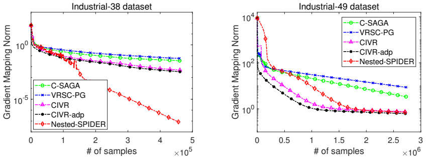
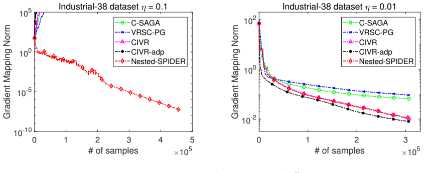
Summary. The paper proposes a Normalized Proximal Approximate Gradient (NPAG) meta-algorithm for nonconvex composite optimization with a possibly nonsmooth convex regularizer, requiring only that the approximate gradients satisfy a mean-squared-error bound that decreases with a prescribed sequence. It then instantiates this framework with SARAH/SPIDER, SVRG, and SAGA estimators under mean-squared Lipschitz or uniform Lipschitz conditions, recovering known one-level complexities. The main contribution is a multi-level Nested-SPIDER method for compositions of expectations or finite sums, for which the paper claims an O~(m^4 L_F (sigma_F^2 + delta_F^2 + l_F^2) epsilon^{-3}) sample complexity in the expectation case and O(sum_i N_i + m^4 L_F sqrt(N_max) epsilon^{-2}) in the finite-sum case, with polynomial rather than exponential dependence on the number of composition levels. Numerical experiments on sparse classification and portfolio selection illustrate the methods.
Significance. If the stated complexities are correct, the paper makes a useful contribution: Theorem 2.3 cleanly separates the optimization dynamics from the stochastic estimation problem, and the nested variance-reduction analysis in Section 4 provides one of the first polynomial-in-m sample complexity results for multi-level composite stochastic optimization, improving on the exponential dependence in previous work such as Yang, Wang, and Fang (2019). The explicit MSE conditions in Theorem 2.3 are stated in terms of problem constants rather than being fitted to the convergence criterion, and the analytical parts of the paper are generally coherent. The main theorems, however, contain arithmetic errors in the sample-accounting steps, and one pseudocode line does not match the analyzed estimator. These issues are local and appear fixable, but they must be corrected before the headline claims can be considered established.
major comments (3)
- [Theorem 4.4, proof (total sample complexity calculation)] The displayed conversion from the per-epoch sums to the final complexity is not algebraically correct. With epsilon_k = m theta L_F / (k l_F), tau_k = l_F / (2m epsilon_k), B_i^k = 12m(m+1) sigma_F^2 / epsilon_k^2, b_i^k = 6(m+1) l_F / epsilon_k, S_i^k = 12m(m+1) delta_F^2 / epsilon_k^2, and s_i^k = 6m(m+1) l_F / epsilon_k, the per-stage cost after summing over i is O(m^3 (sigma_F^2 + delta_F^2) / epsilon_k^2 + m^2 l_F^2 / epsilon_k^2), not the expression printed in the proof. Since sum_{k <= K} epsilon_k^{-2} = O(K^3 l_F^2 / (m^2 L_F^2)) and K = O~(m L_F / (epsilon l_F)), the total is O(m^4 L_F (sigma_F^2 + delta_F^2) / (epsilon^3 l_F) + m^3 L_F l_F / epsilon^3), which differs from the claimed O(m^4 L_F (sigma_F^2 + delta_F^2 + l_F^2) / epsilon^3) by a factor 1/l_F in the first two terms and by a factor m l_F in the last term. The intermediate factor L_F^2 / l_F^2 in the proof should be its reciprocal, and even then the displayed final equality does not follow. The theorem therefore needs a corrected derivation or different parameter choices.
- [Theorem 4.5, proof (epoch count)] The convergence calculation in the proof of Theorem 4.5 gives E[||G(x_bar)||] <= O~( (L_F / (sqrt(N_max) K))^{1/2} ): from equation (48), the dominant term is O(L_F / (N_max^{1/4} sqrt(theta L_F K))) = O((L_F / sqrt(N_max) K)^{1/2}), with the second term smaller up to log factors. Consequently the required number of epochs is K = O~(L_F epsilon^{-2} / sqrt(N_max)), not the printed K = O~(L_F sqrt(N_max) epsilon^{-2}). If the printed epoch count were used, the per-epoch full-batch cost K sum_i N_i alone would be O(m L_F N_max^{3/2} epsilon^{-2}), which is a factor N_max larger than the claimed bound. With the corrected K, the restart cost becomes O(m L_F sqrt(N_max) epsilon^{-2}), consistent with the stated order up to the m-factor. This correction is load-bearing and should be made explicitly.
- [Algorithm 3, else branch] The recursion for y_t^i in the else branch is printed as y_t^i = y_{t-1}^i + f_{i,S_t^i}(y_{t-1}^i) - f'_{i,S_t^i}(y_{t-1}^{t-1}), using the Jacobian f' in the correction term. The analyzed estimator in Lemma 4.3, specifically equations (41) and (44), uses the mapping f_i evaluated at the two points, i.e., the second term should be f_{i,S_t^i}(y_{t-1}^{t-1}). As printed, Algorithm 3 is not the algorithm whose complexity is proven. This is a local typo, but it must be fixed for reproducibility.
minor comments (4)
- [Section 1.2] The contribution summary states that the finite-sum complexity is O(N + m^4 sqrt(N) epsilon^{-1}), but the abstract and Theorem 4.5 state O(N + m^4 L_F sqrt(N_max) epsilon^{-2}); these should be reconciled.
- [Theorem 4.5, proof] The displayed bound on E[||G(x_bar)||] appears with a positive exponent as (L_F sqrt(N_max) K)^{1/2}; it should be (L_F / (sqrt(N_max) K))^{1/2} or equivalently (L_F sqrt(N_max) K)^{-1/2}.
- [Lemma 4.3, Step 4] The induction step uses a Young-type inequality whose coefficients appear in the extracted text as `(1 + k - 1)`; this should be written as (1 + k) and (1 + 1/k) to make the algebra transparent.
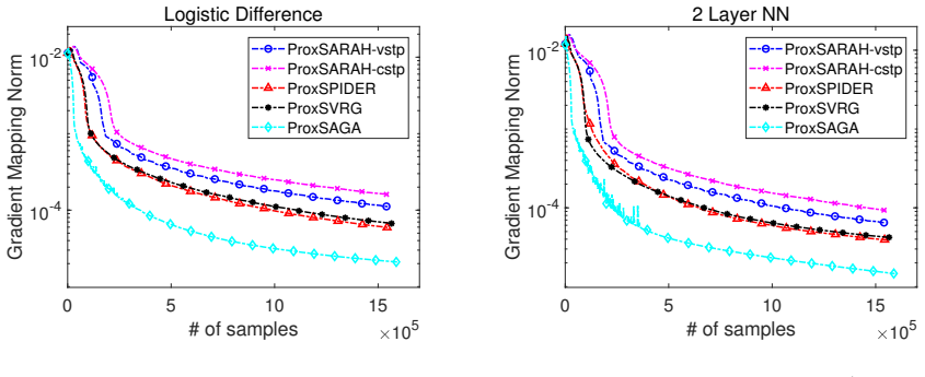
- [Throughout] There are several typographical errors: "Jessen" should be "Jensen" in Theorem 2.3, "precsion" should be "precision" in Section 3, "lager" should be "larger" in Section 3.1, "consevative" should be "conservative" in Remark 4.6, "ProxSIDER" should be "ProxSPIDER" in Section 5.1, and "Jorunal" should be "Journal" in reference [9].
Circularity Check
No significant circularity: the sample-complexity claims are derived from stated smoothness and MSE assumptions, and self-citations are not load-bearing.
full rationale
The central derivation chain is self-contained rather than circular. Theorem 2.3 takes the MSE condition E[||v_t - F'(x_t)||^2] <= eps_t^2 as an algorithmic input and converts it into an iteration complexity for the NPAG method; it does not assume the final stationarity measure. Lemma 4.3 then proves that this MSE condition holds by choosing epoch lengths and batch sizes from problem constants such as Lipschitz parameters and variances, together with the per-stage precision eps_k. Theorem 4.4 sets eps_k = m*theta*L_F/(k*l_F), sums the per-stage sample counts, and solves for the number of epochs K in terms of the target epsilon. The target epsilon enters only at the final K-selection step, not as an input to the MSE construction, and no fitted parameter is renamed as a prediction. The uniform Lipschitz assumption is explicitly stated as a stronger assumption and is a scope restriction rather than a circular import. Self-citations to the authors' prior work appear only in related work and experimental comparisons as baselines; the load-bearing variance-reduction estimate is Lemma 3.1, cited from the external Spider paper [13], and the proximal descent analysis uses standard inequalities. The finite-sum result Theorem 4.5 follows the same template and does not rely on the conclusion being assumed. Any arithmetic or sample-accounting concerns in the displayed complexity lines of Theorems 4.4 and 4.5 are correctness issues, not circularity, because they would not be resolved by assuming the theorem's claimed conclusion. Therefore the paper is self-contained for the circularity pass and scores 0.
Assumptions & free parameters
assumptions (5)
- domain assumption Assumption 2.1: F is differentiable with L-Lipschitz gradient; Ψ is convex and lower-semicontinuous; Φ=F+Ψ is bounded below.
- domain assumption Assumption 4.1(a): for every level i and every realization ξ_i, f_{i,ξ_i} is 𝓁_i-Lipschitz and its Jacobian f'_{i,ξ_i} is L_i-Lipschitz.
- domain assumption Assumption 4.1(b),(c): bounded second moments δ_i^2 and σ_i^2 for f_{i,ξ_i} and f'_{i,ξ_i} around their expectations.
- standard math Standard optimization lemmas: L-smooth descent inequality, strong convexity of the prox subproblem, nonexpansiveness of the proximal operator, Jensen and Young inequalities.
- standard math Lemma 3.1, the SPIDER MSE recursion, is taken from [13, Lemma 1].
Cite this review
Pith. "Pith review of Multi-Level Composite Stochastic Optimization via Nested Variance Reduction." pith.science (2026). https://pith.science/paper/DEA5RWES
@misc{pith2026190811468,
  author       = {Pith},
  title        = {Pith review of: Multi-Level Composite Stochastic Optimization via Nested Variance Reduction},
  year         = {2026},
  howpublished = {\url{https://pith.science/paper/DEA5RWES}},
  note         = {Machine review of arXiv:1908.11468}
}
abstract
We consider multi-level composite optimization problems where each mapping in the composition is the expectation over a family of random smooth mappings or the sum of some finite number of smooth mappings. We present a normalized proximal approximate gradient (NPAG) method where the approximate gradients are obtained via nested stochastic variance reduction. In order to find an approximate stationary point where the expected norm of its gradient mapping is less than $\epsilon$, the total sample complexity of our method is $O(\epsilon^{-3})$ in the expectation case, and $O(N+\sqrt{N}\epsilon^{-2})$ in the finite-sum case where $N$ is the total number of functions across all composition levels. In addition, the dependence of our total sample complexity on the number of composition levels is polynomial, rather than exponential as in previous work.
Figures

Figures from the paper (1 more)
Reference graph
Works this paper leans on
-
[1]
Natasha: Faster non-convex stochastic optimization via strongly non- convex parameter
Zeyuan Allen-Zhu. Natasha: Faster non-convex stochastic optimization via strongly non- convex parameter. In Proceedings of the 34th International Conference on Machine Learning (ICML), volume 70 of Proceedings of Machine Learning Research, pages 89–97, Sydney, Aus- tralia, 2017
work page 2017
-
[2]
Natasha 2: Faster non-convex optimization than SGD
Zeyuan Allen-Zhu. Natasha 2: Faster non-convex optimization than SGD. In Advances in Neural Information Processing Systems 31 , pages 2675–2686. Curran Associates, Inc., 2018. 27
work page 2018
-
[3]
Variance reduction for faster non-convex optimization
Zeyuan Allen-Zhu and Elad Hazan. Variance reduction for faster non-convex optimization. In Proceedings of the 33rd International Conference on Machine Learning , pages 699–707, 2016
work page 2016
-
[4]
Improved SVRG for non-strongly-convex or sum-of-non- convex objectives
Zeyuan Allen-Zhu and Yang Yuan. Improved SVRG for non-strongly-convex or sum-of-non- convex objectives. In Proceedings of the 33rd International Conference on International Con- ference on Machine Learning (ICML) , pages 1080–1089, 2016
work page 2016
-
[5]
First-Order Methods in Optimization
Amir Beck. First-Order Methods in Optimization. MOS-SIAM Series on Optimization. SIAM, 2017
2017
-
[6]
Unbiased simulation for optimizing stochastic function compositions
Jose Blanchet, Donald Goldfarb, Garud Iyengar, Fengpei Li, and Chaoxu Zhou. Unbiased simulation for optimizing stochastic function compositions. Preprint, arXiv:1711.07564, 2017
arXiv 2017
-
[7]
Policy evaluation with temporal dif- ferences: a survey and comparison
Christoph Dann, Gerhard Neumann, and Jan Peters. Policy evaluation with temporal dif- ferences: a survey and comparison. Journal of Machine Learning Research , 15(1):809–883, 2014
work page 2014
-
[8]
SAGA: A fast incremental gradient method with support for non-strongly convex composite objectives
Aaron Defazio, Francis Bach, and Simon Lacoste-Julien. SAGA: A fast incremental gradient method with support for non-strongly convex composite objectives. In Advances in Neural Information Processing Systems 27 , pages 1646–1654, 2014
work page 2014
Show all 43 references
-
[9]
Optimal distributed online prediction using mini-batches
Ofer Dekel, Ran Gilad-Bachrach, Ohad Shamir, and Lin Xiao. Optimal distributed online prediction using mini-batches. Jorunal of Machine Learning Research , 13:165–202, 2012
2012
-
[10]
Statistical estimation of com- posite risk functionals and risk optimization problems
Darinka Dentcheva, Spiridon Penev, and Andrzej Ruszczy´ nski. Statistical estimation of com- posite risk functionals and risk optimization problems. Annals of the Institute of Statistical Mathematics, 69(4):737–760, 2017
2017
-
[11]
Dmitriy Drusvyatskiy and Adrian S. Lewis. Error bounds, quadratic growth, and linear con- vergence of proximal methods. Mathematics of Operations Research, 43(3):919–948, 2018
2018
-
[12]
Ermoliev
Y. Ermoliev. Methods of Stochastic Programming . Monographs in Optimization and OR. Nauka, Moscow, 1976
1976
-
[13]
Spider: Near-optimal non-convex optimization via stochastic path-integrated differential estimator
Cong Fang, Chris Junchi Li, Zhouchen Lin, and Tong Zhang. Spider: Near-optimal non-convex optimization via stochastic path-integrated differential estimator. In Advances in Neural In- formation Processing Systems 31 , pages 689–699. Curran Associates, Inc., 2018
2018
-
[14]
Stochastic first- and zeroth-order methods for nonconvex stochastic programming
Saeed Ghadimi and Guanghui Lan. Stochastic first- and zeroth-order methods for nonconvex stochastic programming. SIAM Journal on Optimization , 23(4):2341–2368, 2013
2013
-
[15]
A single time-scale stochastic ap- proximation method for nested stochastic optimization
Saeed Ghadimi, Andrzej Ruszczy´ nski, and Mengdi Wang. A single time-scale stochastic ap- proximation method for nested stochastic optimization. Preprint, arXiv:1812.01094, 2018
2018 arXiv
-
[16]
Accelerated method for stochastic composi- tion optimization with nonsmooth regularization
Zhouyuan Huo, Bin Gu, Ji Jiu, and Heng Huang. Accelerated method for stochastic composi- tion optimization with nonsmooth regularization. In Proceedings of the 32nd AAAI Conference on Artificial Intelligence , pages 3287–3294, 2018
2018
-
[17]
A. N. Iusem, A. Jofr´ e, R. I. Oliveira, and P. Phompson. Extragradient method with variance reduction for stochastic variational inequalities. SIAM Journal on Optimization , 27(2):686– 724, 2017. 28
2017
-
[18]
Accelerating stochastic gradient descent using predictive vari- ance reduction
Rie Johnson and Tong Zhang. Accelerating stochastic gradient descent using predictive vari- ance reduction. In Advances in Neural Information Processing Systems 26 , pages 315–323, 2013
2013
-
[19]
Koshal, A
J. Koshal, A. Nedi´ c, and U. B. Shanbhag. Regularized iterative stochastic approximation methods for stochastic variational inequality problems. IEEE Transactions on Automatic Control, 58(3):594–609, 2013
2013
-
[20]
Finite-sum composition optimization via variance reduced gradient descent
Xiangru Lian, Mengdi Wang, and Ji Liu. Finite-sum composition optimization via variance reduced gradient descent. In Proceedings of the 20th International Conference on Artificial Intelligence and Statistics (AISTATS) , pages 1159–1167, 2017
2017
-
[21]
Improved oracle complexity for stochastic compositional variance reduced gradient
Tianyi Lin, Chenyou Fan, Mengdi Wang, and Michael I Jordan. Improved oracle complexity for stochastic compositional variance reduced gradient. Preprint, arXiv:1806.00458, 2018
2018 arXiv
-
[22]
Gradient methods for minimizing composite functions
Yurii Nesterov. Gradient methods for minimizing composite functions. Mathematical Pro- gramming, 140(1):125–161, 2013
2013
-
[23]
Lectures on Convex Optimization
Yurii Nesterov. Lectures on Convex Optimization . Springer, 2nd edition, 2018
2018
-
[24]
Nguyen, Jie Liu, Katya Scheinberg, and Martin Tak´ aˇ c
Lam M. Nguyen, Jie Liu, Katya Scheinberg, and Martin Tak´ aˇ c. SARAH: A novel method for machine learning problems using stochastic recursive gradient. In Proceedings of the 34th International Conference on Machine Learning (ICML), volume 70 ofPMLR, pages 2613–2621, 2017
2017
-
[25]
Nguyen, Marten van Dijk, Dzung T
Lam M. Nguyen, Marten van Dijk, Dzung T. Phan, Phuong Ha Nguyen, Tsui-Wei Weng, and Jayant R. Kalagnanam. Finite-sum smooth optimization with SARAH. arXiv:1901.07648, 2019
1901 arXiv
-
[26]
Pham, Lam M
Nhan H. Pham, Lam M. Nguyen, Dzung T. Phan, and Quoc Tran-Dinh. ProxSARAH: An efficient algorithmic framework for stochastic composite nonconvex optimization. Preprint, arXiv:1902.05679, 2019
1902 arXiv
-
[27]
Reddi, Ahmed Hefny, Suvrit Sra, Barnabas Poczos, and Alex Smola
Sashank J. Reddi, Ahmed Hefny, Suvrit Sra, Barnabas Poczos, and Alex Smola. Stochastic variance reduction for nonconvex optimization. In Proceedings of The 33rd International Con- ference on Machine Learning, volume 48 of Proceedings of Machine Learning Research, pages 314–323...
2016
-
[28]
Fast incremental method for smooth nonconvex optimization
Sashank J Reddi, Suvrit Sra, Barnab´ as P´ oczos, and Alex Smola. Fast incremental method for smooth nonconvex optimization. In 2016 IEEE 55th Conference on Decision and Control (CDC), pages 1971–1977. IEEE, 2016
2016
-
[29]
Proximal stochastic methods for nonsmooth nonconvex finite-sum optimization
Sashank J Reddi, Suvrit Sra, Barnab´ as P´ oczos, and Alexander J Smola. Proximal stochastic methods for nonsmooth nonconvex finite-sum optimization. InAdvances in Neural Information Processing Systems 29, pages 1145–1153, 2016
2016
-
[30]
Tyrrell Rockafellar
R. Tyrrell Rockafellar. Convex Analysis. Princeton University Press, 1970
1970
-
[31]
Tyrrell Rockafellar
R. Tyrrell Rockafellar. Coherent approaches to risk in optimization under uncertainty. IN- FORMS TutORials in Operations Research, 2007. 29
2007
-
[32]
Roux, Mark Schmidt, and Francis R
Nicolas L. Roux, Mark Schmidt, and Francis R. Bach. A stochastic gradient method with an exponential convergence rate for finite training sets. In Advances in Neural Information Processing Systems 25, pages 2663–2671. Curran Associates, Inc., 2012
2012
-
[33]
Advances in risk-averse optimization.INFORMS TutORials in Operation Research, 2013
Andrzej Ruszczy´ nski. Advances in risk-averse optimization.INFORMS TutORials in Operation Research, 2013
2013
-
[34]
Reinforcement Learning: An Introduction
Richard S Sutton and Andrew G Barto. Reinforcement Learning: An Introduction. MIT Press, Cambridge, MA, 1998
1998
-
[35]
Stochastic compositional gradient descent: algo- rithms for minimizing compositions of expected-value functions
Mengdi Wang, Ethan X Fang, and Han Liu. Stochastic compositional gradient descent: algo- rithms for minimizing compositions of expected-value functions. Mathematical Programming, 161(1-2):419–449, 2017
2017
-
[36]
Accelerating stochastic composition optimization
Mengdi Wang, Ji Liu, and Ethan Fang. Accelerating stochastic composition optimization. Journal of Machine Learning Research , 18(105):1–23, 2017
2017
-
[37]
SpiderBoost: A class of faster variance-reduced algorithms for nonconvex optimization
Zhe Wang, Kaiyi Ji, Yi Zhou, Yingbin Liang, and Vahid Tarokh. SpiderBoost: A class of faster variance-reduced algorithms for nonconvex optimization. Preprint, arXiv:1810.10690, 2018
2018 arXiv
-
[38]
A proximal stochastic gradient method with progressive variance reduction
Lin Xiao and Tong Zhang. A proximal stochastic gradient method with progressive variance reduction. SIAM Journal on Optimization , 24(4):2057–2075, 2014
2014
-
[39]
Shuoguang Yang, Mengdi Wang, and Ethan X. Fang. Multilevel stochastic gradient methods for nested composition optimization. SIAM Journal on Optimization , 29(1):616–659, 2019
2019
-
[40]
Adversarial examples: Attacks and defenses for deep learning
Xiaoyong Yuan, Pan He, Qile Zhu, and Xiaolin Li. Adversarial examples: Attacks and defenses for deep learning. IEEE Transactions on Neural Networks and Learning Systems , 30(9):2805– 2824, 2019
2019
-
[41]
A composite randomized incremental gradient method
Junyu Zhang and Lin Xiao. A composite randomized incremental gradient method. In Pro- ceedings of the 36th International Conference on Machine Learning (ICML) , number 97 in Proceedings of Machine Learning Research (PMLR), Long Beach, California, 2019
2019
-
[42]
A stochastic composite gradient method with incremental variance reduction
Junyu Zhang and Lin Xiao. A stochastic composite gradient method with incremental variance reduction. In Advances in Neural Information Processing Systems 32, pages 9078–9088. Curran Associates, Inc., 2019
2019
-
[43]
Stochastic nested variance reduced gradient descent for nonconvex optimization
Dongruo Zhou, Pan Xu, and Quanquan Gu. Stochastic nested variance reduced gradient descent for nonconvex optimization. In Advances in Neural Information Processing Systems 31, pages 3921–3932. Curran Associates, Inc., 2018. 30
2018
Reviewed August 14, 2026 · model on record in the stance chip above.
Discussion (0). Continue with ORCID to comment.