REVIEW 3 major objections 5 minor 48 references
Directionally Constrained Fully Convolutional Neural Network For Airborne Lidar Point Cloud Classification
T0 review · 3 major / 5 minor · reviewed 2026-08-14 · deepseek-v4-flash
Pith's one-line read This paper claims that a directionally constrained convolutional network, using only raw coordinates and intensity, sets a new state of the art for airborne LiDAR point cloud classification with 70.7% average F1 on the ISPRS benchmark.
desk verdict The D-Conv module is a genuine contribution, but the state-of-the-art claim is unsupported because hyperparameters were selected on the test set and the reported F1 is the best grid value. read the letter →
The pith
A machine-rendered reading of the paper's core claim, the machinery that carries it, and where it could break.
The reading
What carries the argument
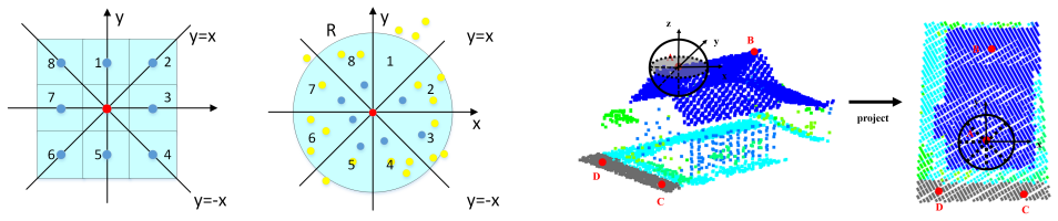
The central object is the directionally constrained point convolution (D-Conv) module. For each central point it partitions the projected xy-plane into Nd=8 triangular sectors, searches K nearest neighbors inside a radius R in each sector (duplicating the central point for empty sectors), and concatenates the sectors in fixed order around the point. A 1×K convolution aggregates each sector's K neighbors into one direction-aware feature, then a 1×Nd convolution combines the Nd directional features into the output, with a residual connection. This fixed sector ordering is what lets the module apply convolution to unordered point sets while preserving local orientation, and the xy-plane (rather than 3D cone) partition is what keeps the receptive fields populated for airborne scans. Around this module, the network uses farthest-point downsampling and distance-based upsampling blocks to build multiscale features, and skip connections to retain low-level detail.
What would settle it
Hold out a validation split within Scene I, or tune on Scene II and evaluate once on Scene III, then rerun the hyperparameter search; if the average F1 drops substantially below 70.7%, the reported state-of-the-art gap is partly an artifact of test-set selection.
Extended reading notes
Core claim
The paper's central claim is that imposing a fixed directional order on point-cloud neighborhoods makes convolutional feature learning more effective for airborne LiDAR. Concretely, D-FCN projects the neighborhood of each point onto the xy plane, divides it into eight 45-degree sectors, picks K nearest neighbors in each sector, and uses the sector order as the channel order of a convolution. This orientation-aware operator, stacked in a U-shaped fully convolutional network with downsampling and upsampling blocks, yields 82.2% overall accuracy and 70.7% average F1 on the ISPRS benchmark using only x, y, z and intensity as input, an average F1 above the previous best method and with large gains on the powerline, car, and facade classes. The paper also shows by ablation that the 2D eight-direction search outperforms both no directional partition and an eight-direction search in 3D.
Load-bearing premise
The paper tunes its hyperparameters on the same ISPRS test set that it then uses to report the final 70.7% average F1, so the headline number may be inflated by selection bias.
Editorial extensions
If this is right
- Airborne LiDAR classification pipelines can be built without computing handcrafted geometric features such as planarity, sphericity, or roughness; raw x, y, z and intensity are sufficient for the reported accuracy.
- The fully convolutional design lets whole test blocks be processed in one forward pass, so practical systems can label scenes of arbitrary point count without per-point inference.
- Direction-aware receptive fields improve minority classes: compared with prior methods, powerline F1 rises 8.4 points, car 3.4, and facade 7.3, on the ISPRS benchmark.
- On this benchmark, optimizing hyperparameters for average F1 instead of overall accuracy trades roughly three points of overall accuracy (82.2% versus 85.2%) for a better balance across categories, so the right metric depends on whether the application needs rare-class recall or bulk accuracy.
Reading between the lines
- My inference: the directional-sector idea is not tied to airborne LiDAR; projecting onto a local dominant plane instead of the xy plane would extend D-Conv to mobile or indoor point clouds, where vertical structure is richer than horizontal spread.
- My inference: because sector order is defined in world x-y coordinates, the learned filters depend on the scanner's heading; an orientation-normalization or rotation-augmentation step could make the network invariant to flight direction and would isolate the contribution of ordering.
- My inference: the rare-class improvements could come from the class-balanced loss, the directional convolution, or both; ablating the two factors separately on the same benchmark would apportion the gain.
- My inference: D-Conv is a generic convolution operator for unordered point sets, so it could be dropped into other point-based architectures for tasks like powerline extraction or building facade detection, where rare elongated classes matter.
Signed reviews
Editorial analysis
A structured set of objections, weighed in public.
Referee Report
Summary. This paper proposes D-FCN, a fully convolutional neural network for semantic segmentation of airborne LiDAR point clouds. The key component is a directionally constrained point convolution (D-Conv) module that projects points onto the xy-plane, partitions the plane into eight angular sectors, and performs a K-nearest-neighbor search within each sector to build an ordered receptive field; feature aggregation is then performed via 1xK and 1xNd convolutions. Experiments on the ISPRS 3D labeling benchmark report an average F1 of 70.7% and overall accuracy of 82.2%, which the authors claim is a new state-of-the-art average F1. The paper includes ablations over the number of directional sectors, the number of sampled points N, the number of neighbors K, and the class-balance coefficient alpha.
Significance. If the reported performance were obtained under an unbiased protocol, the D-Conv design (orientation-aware grouping on the projected 2D space) would be a modest but useful contribution for airborne LiDAR classification, especially for minority classes such as powerline, car, and facade. The paper provides extensive ablation tables and a comparison with eight prior ISPRS methods, which is a valuable empirical study. However, the central empirical claim is compromised by the fact that all hyperparameters were selected on the official test set, so the headline 70.7% average F1 is likely optimistically biased; the claimed advantage over the prior best (NANJ2) is only 1.4 percentage points, which is smaller than the variation across hyperparameter settings in Table 3. The significance of the paper therefore depends on whether the authors can re-establish the result with a proper validation split.
major comments (3)
- [Section 4.5, Tables 3 and 4] The state-of-the-art claim is not supported because hyperparameters are selected on the test set. Section 4.5 explicitly states that "Average F1 score was adopted as the evaluation metric to select the best hyperparameters," and Tables 3 and 4 are computed on the official test scenes (Scene II and III). The final configuration (N=8192, K=2, alpha=1.2) is simply the maximum of a grid search over 12 (N,K) combinations and 6 alpha values, evaluated on the same data used for the final comparison in Table 6. This is a form of test-set overfitting. The problem is compounded by the small claimed margin: the range of average F1 in Table 3 (0.679-0.707) is about twice the reported advantage over NANJ2 (0.707-0.693 = 0.014), so the best configuration may well be a lucky draw. The authors must either (i) use a validation set (e.g., a hold-out part of Scene I) for hyperparameter selection and report results on the test set only once, or (ii) provide a corrected analysis that accounts for the selection bias. As it stands, the paper's Section 4.1 statement that test labels "were used only for model evaluation" is contradicted by the procedure in Section 4.5.
- [Section 4.6 and Table 6] The comparison with prior work is also affected by the choice of metric. The paper reports an OA of 82.2%, which is 3.0 points below NANJ2 (85.2%) and 2.7 points below WhuY4 (84.9%). The authors acknowledge in Section 4.7 that many hyperparameter settings yield higher OA (up to 84.6%) but were discarded because average F1 was prioritized. This makes explicit that the final model was selected by optimizing the exact metric used for the SOTA claim on the test set. For a fair benchmark comparison, the evaluation metric and the model-selection rule should be fixed before seeing test labels, and the final result should be reported as a single evaluation rather than the best among many test-set evaluations.
- [Section 4.5, Tables 3-4] The paper provides no measure of variance or reproducibility (e.g., multiple independent runs with different random seeds). Given that Table 3 shows a 2.8-percentage-point difference between the worst (0.679) and best (0.707) configurations and that the claimed improvement over the previous best is only 1.4 points, it is possible that the reported advantage is not statistically distinguishable from run-to-run variation. The authors should report mean and standard deviation over repeated runs (at least for the final configuration) and, ideally, perform a significance test against the closest competitor.
minor comments (5)
- [Section 3.2.2] The sentence "We insert our D-Conv module is inserted before each downsampling operation" contains a duplicated verb and should be corrected to "We insert our D-Conv module before each downsampling operation."
- [Section 3.2.2] The phrase "The low level-level features" should be corrected to "The low-level features."
- [Abstract and Conclusion] The claim of a "new state-of-the-art level of performance" should be qualified as "in terms of average F1 score" to avoid the misleading impression that the method also achieves the best overall accuracy, since the reported OA (82.2%) is lower than several competing methods.
- [Section 4.2, Equation (6)] The class-balance weighting is not fully specified for the "no balancing" case (alpha = NA in Table 4); the authors should state explicitly what weight is used when no balancing is applied (presumably W_c = 1).
- [Table 5] The confusion matrix is presented row-wise as the distribution of true labels, but the caption does not state the convention; please clarify that rows are ground truth and columns are predictions (or vice versa).
Circularity Check
The reported 70.7% average F1 is not an unbiased prediction: the same test split is used to select N, K, alpha, and the 2D 8-direction partition by maximizing F1, and the final result is the best value of that grid search.
-
fitted input called prediction
[Section 4.5 (Model hyperparameters), including Section 4.5.1, Section 4.5.2, Tables 3-4; reported again in Section 4.6/Table 5]
"Average F1 score was adopted as the evaluation metric to select the best hyperparameters. ... Our model achieved its best performance when N and K were set to 8,192 and 2, respectively, with an overall accuracy of 82.2% and an average F1 score of 70.7%. Hereafter, we use this configuration for N and K in our experiments. ... The highest average F1 score of 70.7% was achieved by the model where the class balance coefficient α was set to 1.2. ... Note that the test dataset labels were used only for model evaluation, which is unknown during the model training stage."
The reported SOTA number is the same quantity used as the selection objective. Section 4.5 chooses N, K, and alpha by the average F1 achieved on the test scenes (Tables 3 and 4), and Section 4.4 chooses the 2D 8-direction partition in the same way (Table 2). Section 4.6 then reports exactly the best configuration's test F1 (70.7%) as the final 'state-of-the-art' result and uses it in Table 6 against fixed prior methods. Since no validation split or nested CV is used, the headline number is the maximum of a grid over the test set, not an unbiased prediction. The margin over NANJ2 (0.707 vs 0.693) is smaller than the 0.028 spread across Table 3, so test-set selection can fully explain the claimed improvement.
full rationale
The paper is an empirical benchmark paper, not a first-principles derivation. The D-Conv equations (1)-(2), the downsampling/upsampling architecture, and the loss (7) are specified independently of the result; there is no self-citation chain or definitional identification of the architecture with the output metric. The core numerical claim, however, is partially circular in the statistical sense: hyperparameters and the directional partition are selected by maximizing the same test-set F1 that is later reported as the achieved performance. The final configuration is the argmax of a grid over the test split, so the 70.7% figure is a fitted maximum rather than a held-out estimate. Because the architecture is still compared to prior methods on the same benchmark and the comparison is not itself derived from the fitted value, the circularity is partial rather than total. Score 6 per the rubric: one or more 'predictions' reduce by construction to test-set selection.
Assumptions & free parameters
free parameters (6)
- N (sampling points per training block) =
8192
- K (neighbor points per directional sector) =
2
- alpha (class balance coefficient) =
1.2
- Nd (number of directional sectors) =
8 (2D space)
- Search radii R at each downsampling level =
2, 5, 10
- Dropout ratio =
12.5%
assumptions (4)
- domain assumption xy-projected angular partition preserves sufficient local structure for classifying airborne LiDAR points
- domain assumption Central-point duplication in empty sectors is a valid filler for absent neighbors
- domain assumption Test set can be used for hyperparameter selection and still yield an unbiased estimate of performance
- standard math Farthest point sampling and inverse-distance interpolation from PointNet++ are valid for multiscale downsampling and upsampling
Cite this review
Pith. "Pith review of Directionally Constrained Fully Convolutional Neural Network For Airborne Lidar Point Cloud Classification." pith.science (2026). https://pith.science/paper/DHYMTYJ5
@misc{pith2026190806673,
  author       = {Pith},
  title        = {Pith review of: Directionally Constrained Fully Convolutional Neural Network For Airborne Lidar Point Cloud Classification},
  year         = {2026},
  howpublished = {\url{https://pith.science/paper/DHYMTYJ5}},
  note         = {Machine review of arXiv:1908.06673}
}
read the original abstract
Point cloud classification plays an important role in a wide range of airborne light detection and ranging (LiDAR) applications, such as topographic mapping, forest monitoring, power line detection, and road detection. However, due to the sensor noise, high redundancy, incompleteness, and complexity of airborne LiDAR systems, point cloud classification is challenging. In this paper, we proposed a directionally constrained fully convolutional neural network (D-FCN) that can take the original 3D coordinates and LiDAR intensity as input; thus, it can directly apply to unstructured 3D point clouds for semantic labeling. Specifically, we first introduce a novel directionally constrained point convolution (D-Conv) module to extract locally representative features of 3D point sets from the projected 2D receptive fields. To make full use of the orientation information of neighborhood points, the proposed D-Conv module performs convolution in an orientation-aware manner by using a directionally constrained nearest neighborhood search. Then, we designed a multiscale fully convolutional neural network with downsampling and upsampling blocks to enable multiscale point feature learning. The proposed D-FCN model can therefore process input point cloud with arbitrary sizes and directly predict the semantic labels for all the input points in an end-to-end manner. Without involving additional geometry features as input, the proposed method has demonstrated superior performance on the International Society for Photogrammetry and Remote Sensing (ISPRS) 3D labeling benchmark dataset. The results show that our model has achieved a new state-of-the-art level of performance with an average F1 score of 70.7%, and it has improved the performance by a large margin on categories with a small number of points (such as powerline, car, and facade).
Figures


Figures from the paper (6 more)


Reference graph
Works this paper leans on
-
[1]
Andersen, H.-E., McGaughey, R. J. and Reutebuch, S. E., 2005. Estimating forest canopy fuel parameters using lidar data. Remote sensing of Environment 94(4), pp. 441--449
work page 2005
-
[2]
Dem generation from laser scanner data using adaptive tin models
Axelsson, P., 2000. Dem generation from laser scanner data using adaptive tin models. International archives of photogrammetry and remote sensing 33(4), pp. 110--117
work page 2000
-
[3]
Babahajiani, P., Fan, L., K \"a m \"a r \"a inen, J.-K. and Gabbouj, M., 2017. Urban 3d segmentation and modelling from street view images and lidar point clouds. Machine Vision and Applications 28(7), pp. 679--694
work page 2017
-
[4]
Badrinarayanan, V., Kendall, A. and Cipolla, R., 2017. Segnet: A deep convolutional encoder-decoder architecture for image segmentation. IEEE transactions on pattern analysis and machine intelligence 39(12), pp. 2481--2495
work page 2017
-
[5]
Chan, T.-H., Jia, K., Gao, S., Lu, J., Zeng, Z. and Ma, Y., 2015. Pcanet: A simple deep learning baseline for image classification? IEEE transactions on image processing 24(12), pp. 5017--5032
work page 2015
-
[6]
Chehata, N., Guo, L. and Mallet, C., 2009. Airborne lidar feature selection for urban classification using random forests. International Archives of Photogrammetry, Remote Sensing and Spatial Information Sciences 38(Part 3), pp. W8
work page 2009
-
[7]
Collobert, R. and Weston, J., 2008. A unified architecture for natural language processing: Deep neural networks with multitask learning. In: Proceedings of the 25th international conference on Machine learning, ACM, pp. 160--167
work page 2008
-
[8]
The dgpf-test on digital airborne camera evaluation--overview and test design
Cramer, M., 2010. The dgpf-test on digital airborne camera evaluation--overview and test design. Photogrammetrie-Fernerkundung-Geoinformation 2010(2), pp. 73--82
work page 2010
Show all 48 references
-
[9]
T., N sset, E., Gobakken, T., Bollands s, O
Ene, L. T., N sset, E., Gobakken, T., Bollands s, O. M., Mauya, E. W. and Zahabu, E., 2017. Large-scale estimation of change in aboveground biomass in miombo woodlands using airborne laser scanning and national forest inventory data. Remote Sensing of Environment 188, pp. 106--117
2017
-
[10]
et al., 2012
Hinton, G., Deng, L., Yu, D., Dahl, G., Mohamed, A.-r., Jaitly, N., Senior, A., Vanhoucke, V., Nguyen, P., Kingsbury, B. et al., 2012. Deep neural networks for acoustic modeling in speech recognition. IEEE Signal processing magazine
2012
-
[11]
and Mongus, D., 2016
Horvat, D., Z alik, B. and Mongus, D., 2016. Context-dependent detection of non-linearly distributed points for vegetation classification in airborne lidar. ISPRS Journal of Photogrammetry and Remote Sensing 116, pp. 1--14
2016
-
[12]
and Lu, C., 2018
Jiang, M., Wu, Y. and Lu, C., 2018. Pointsift: A sift-like network module for 3d point cloud semantic segmentation. arXiv preprint arXiv:1807.00652
2018 arXiv
-
[13]
and McKinley, L., 2009
Kada, M. and McKinley, L., 2009. 3d building reconstruction from lidar based on a cell decomposition approach. International Archives of Photogrammetry, Remote Sensing and Spatial Information Sciences 38(Part 3), pp. W4
2009
-
[14]
and Hebert, M., 2005
Lalonde, J.-F., Unnikrishnan, R., Vandapel, N. and Hebert, M., 2005. Scale selection for classification of point-sampled 3d surfaces. In: Fifth International Conference on 3-D Digital Imaging and Modeling (3DIM'05), IEEE, pp. 285--292
2005
-
[15]
Lalonde, J.-F., Vandapel, N., Huber, D. F. and Hebert, M., 2006. Natural terrain classification using three-dimensional ladar data for ground robot mobility. Journal of field robotics 23(10), pp. 839--861
2006
-
[16]
and Hinton, G., 2015
LeCun, Y., Bengio, Y. and Hinton, G., 2015. Deep learning. nature 521(7553), pp. 436
2015
-
[17]
and Chi, T., 2016
Li, X., Peng, L., Hu, Y., Shao, J. and Chi, T., 2016. Deep learning architecture for air quality predictions. Environmental Science and Pollution Research 23(22), pp. 22408--22417
2016
-
[18]
and Fang, Y., 2018
Li, X., Yao, X. and Fang, Y., 2018. Building-a-nets: Robust building extraction from high-resolution remote sensing images with adversarial networks. IEEE Journal of Selected Topics in Applied Earth Observations and Remote Sensing (99), pp. 1--8
2018
-
[19]
K., Fitzpatrick, D
Lodha, S. K., Fitzpatrick, D. M. and Helmbold, D. P., 2007. Aerial lidar data classification using adaboost. In: Sixth International Conference on 3-D Digital Imaging and Modeling (3DIM 2007), IEEE, pp. 435--442
2007
-
[20]
and Hensman, P., 2015
Masko, D. and Hensman, P., 2015. The impact of imbalanced training data for convolutional neural networks
2015
-
[21]
and Z alik, B., 2013
Mongus, D. and Z alik, B., 2013. Computationally efficient method for the generation of a digital terrain model from airborne lidar data using connected operators. IEEE journal of selected topics in applied earth observations and remote sensing 7(1), pp. 340--351
2013
-
[22]
A., Vandapel, N
Munoz, D., Bagnell, J. A., Vandapel, N. and Hebert, M., 2009. Contextual classification with functional max-margin markov networks. In: 2009 IEEE Conference on Computer Vision and Pattern Recognition, IEEE, pp. 975--982
2009
-
[23]
and Soergel, U., 2012
Niemeyer, J., Rottensteiner, F. and Soergel, U., 2012. Conditional random fields for lidar point cloud classification in complex urban areas. ISPRS annals of the photogrammetry, remote sensing and spatial information sciences 3, pp. 263--268
2012
-
[24]
and Soergel, U., 2014
Niemeyer, J., Rottensteiner, F. and Soergel, U., 2014. Contextual classification of lidar data and building object detection in urban areas. ISPRS journal of photogrammetry and remote sensing 87, pp. 152--165
2014
-
[25]
and Heipke, C., 2016
Niemeyer, J., Rottensteiner, F., S \"o rgel, U. and Heipke, C., 2016. Hierarchical higher order crf for the classification of airborne lidar point clouds in urban areas. International Archives of the Photogrammetry, Remote Sensing and Spatial Information Sciences-ISPRS Archive...
2016
-
[26]
R., Su, H., Mo, K
Qi, C. R., Su, H., Mo, K. and Guibas, L. J., 2017a. Pointnet: Deep learning on point sets for 3d classification and segmentation. In: Proceedings of the IEEE Conference on Computer Vision and Pattern Recognition, pp. 652--660
-
[27]
R., Su, H., Nie ner, M., Dai, A., Yan, M
Qi, C. R., Su, H., Nie ner, M., Dai, A., Yan, M. and Guibas, L. J., 2016. Volumetric and multi-view cnns for object classification on 3d data. In: Proceedings of the IEEE conference on computer vision and pattern recognition, pp. 5648--5656
2016
-
[28]
R., Yi, L., Su, H
Qi, C. R., Yi, L., Su, H. and Guibas, L. J., 2017b. Pointnet++: Deep hierarchical feature learning on point sets in a metric space. In: Advances in Neural Information Processing Systems, pp. 5099--5108
-
[29]
and Vosselmann, G., 2006
Rabbani, T., Van Den Heuvel, F. and Vosselmann, G., 2006. Segmentation of point clouds using smoothness constraint. International archives of photogrammetry, remote sensing and spatial information sciences 36(5), pp. 248--253
2006
-
[30]
and Brox, T., 2015
Ronneberger, O., Fischer, P. and Brox, T., 2015. U-net: Convolutional networks for biomedical image segmentation. In: International Conference on Medical image computing and computer-assisted intervention, Springer, pp. 234--241
2015
-
[31]
and Barinova, O., 2010
Shapovalov, R., Velizhev, E. and Barinova, O., 2010. Nonassociative markov networks for 3d point cloud classification. the. In: International Archives of the Photogrammetry, Remote Sensing and Spatial Information Sciences XXXVIII, Part 3A, Citeseer
2010
-
[32]
and Tian, D., 2018
Shen, Y., Feng, C., Yang, Y. and Tian, D., 2018. Mining point cloud local structures by kernel correlation and graph pooling. In: Proceedings of the IEEE conference on computer vision and pattern recognition, pp. 4548--4557
2018
-
[33]
H., Lange, H., N sset, E., Rautiainen, M
Solberg, S., Brunner, A., Hanssen, K. H., Lange, H., N sset, E., Rautiainen, M. and Stenberg, P., 2009. Mapping lai in a norway spruce forest using airborne laser scanning. Remote Sensing of Environment 113(11), pp. 2317--2327
2009
-
[34]
and Learned-Miller, E., 2015
Su, H., Maji, S., Kalogerakis, E. and Learned-Miller, E., 2015. Multi-view convolutional neural networks for 3d shape recognition. In: Proceedings of the IEEE international conference on computer vision, pp. 945--953
2015
-
[35]
and Rottensteiner, F., 2017
Vosselman, G., Coenen, M. and Rottensteiner, F., 2017. Contextual segment-based classification of airborne laser scanner data. ISPRS journal of photogrammetry and remote sensing 128, pp. 354--371
2017
-
[36]
E., Bronstein, M
Wang, Y., Sun, Y., Liu, Z., Sarma, S. E., Bronstein, M. M. and Solomon, J. M., 2018a. Dynamic graph cnn for learning on point clouds. arXiv preprint arXiv:1801.07829
-
[37]
and Zhu, Z., 2018b
Wang, Z., Zhang, L., Zhang, L., Li, R., Zheng, Y. and Zhu, Z., 2018b. A deep neural network with spatial pooling (dnnsp) for 3-d point cloud classification. IEEE Transactions on Geoscience and Remote Sensing 56(8), pp. 4594--4604
-
[38]
and Mallet, C., 2015a
Weinmann, M., Jutzi, B., Hinz, S. and Mallet, C., 2015a. Semantic point cloud interpretation based on optimal neighborhoods, relevant features and efficient classifiers. ISPRS Journal of Photogrammetry and Remote Sensing 105, pp. 286--304
-
[39]
and Jutzi, B., 2015b
Weinmann, M., Schmidt, A., Mallet, C., Hinz, S., Rottensteiner, F. and Jutzi, B., 2015b. Contextual classification of point cloud data by exploiting individual 3d neigbourhoods. ISPRS Annals of the Photogrammetry, Remote Sensing and Spatial Information Sciences II-3 (2015), Nr...
2015
-
[40]
and Chi, T., 2019
Wen, C., Liu, S., Yao, X., Peng, L., Li, X., Hu, Y. and Chi, T., 2019. A novel spatiotemporal convolutional long short-term neural network for air pollution prediction. Science of The Total Environment 654, pp. 1091--1099
2019
-
[41]
and Zhong, R., 2017a
Yang, B., Huang, R., Li, J., Tian, M., Dai, W. and Zhong, R., 2017a. Automated reconstruction of building lods from airborne lidar point clouds using an improved morphological scale space. Remote Sensing 9(1), pp. 14
-
[42]
and Huang, W., 2017b
Yang, Z., Jiang, W., Xu, B., Zhu, Q., Jiang, S. and Huang, W., 2017b. A convolutional neural network-based 3d semantic labeling method for als point clouds. Remote Sensing 9(9), pp. 936
-
[43]
and Jiang, W., 2018
Yang, Z., Tan, B., Pei, H. and Jiang, W., 2018. Segmentation and multi-scale convolutional neural network-based classification of airborne laser scanner data. Sensors 18(10), pp. 3347
2018
-
[44]
J., Ientilucci, E
Yousefhussien, M., Kelbe, D. J., Ientilucci, E. J. and Salvaggio, C., 2018. A multi-scale fully convolutional network for semantic labeling of 3d point clouds. ISPRS journal of photogrammetry and remote sensing 143, pp. 191--204
2018
-
[45]
and Ning, X., 2013
Zhang, J., Lin, X. and Ning, X., 2013. Svm-based classification of segmented airborne lidar point clouds in urban areas. Remote Sensing 5(8), pp. 3749--3775
2013
-
[46]
and Popescu, S., 2009
Zhao, K. and Popescu, S., 2009. Lidar-based mapping of leaf area index and its use for validating globcarbon satellite lai product in a temperate forest of the southern usa. Remote Sensing of Environment 113(8), pp. 1628--1645
2009
-
[47]
and Wang, J., 2018
Zhao, R., Pang, M. and Wang, J., 2018. Classifying airborne lidar point clouds via deep features learned by a multi-scale convolutional neural network. International Journal of Geographical Information Science 32(5), pp. 960--979
2018
-
[48]
and Wu, B., 2017
Zhu, Q., Li, Y., Hu, H. and Wu, B., 2017. Robust point cloud classification based on multi-level semantic relationships for urban scenes. ISPRS Journal of Photogrammetry and Remote Sensing 129, pp. 86--102
2017
Reviewed August 14, 2026 · model on record in the stance chip above.
Discussion (0). Continue with ORCID to comment.