REVIEW 3 major objections 4 minor 23 references
Taxonomy of amorphous ternary phase diagrams: the importance of interaction parameters
T0 review · 3 major / 4 minor · reviewed 2026-08-10 · deepseek-v4-flash
Pith's one-line read A taxonomy of 21 ternary phase diagram types from 80,000 simulations
desk verdict A useful systematic catalog of ternary Flory-Huggins diagrams whose common-type taxonomy is likely robust, but the rare types that carry much of the novelty sit exactly where the paper's own classification heuristic is admitted to be ill-defined, and no sensitivity analysis is provided. read the letter →
The pith
A machine-rendered reading of the paper's core claim, the machinery that carries it, and where it could break.
The reading
What carries the argument
The load-bearing objects are the pair-critical interaction parameter, $\chi^c_{ij}=\frac{1}{2}\bigl(1/\sqrt{N_i}+1/\sqrt{N_j}\bigr)^2$, and the normalized coordinates $\bar\chi_{ij}=\chi_{ij}/\chi^c_{ij}$, whose unit planes partition the design space into octants. Phase diagrams are computed from the lattice free-energy model $\Delta G/(RT/v_0)=\sum_i \phi_i\ln\phi_i/N_i+\sum_{i<j}\phi_i\phi_j\chi_{ij}$ by discretizing the composition triangle on a 300-point grid, constructing the lower convex hull of the free-energy surface, and projecting the elongated hull triangles back to composition space to mark two- and three-phase regions. A connected-components labeling then assigns each diagram a three-digit key (number of one-, two-, and three-phase regions), and that key is the taxonomy's classifier. The octant map in normalized parameter space is the rule engine that connects parameter values to diagram type.
What would settle it
Recompute the rarest reported type ([463]), found only once among 81,000 diagrams in a narrow near-critical window, with an independent free-energy-minimization or tie-line solver on much finer grids; if the three-phase topology does not reproduce, that rare type is an artifact of the convex-hull classification rather than a genuine thermodynamic phase-diagram class.
Extended reading notes
Core claim
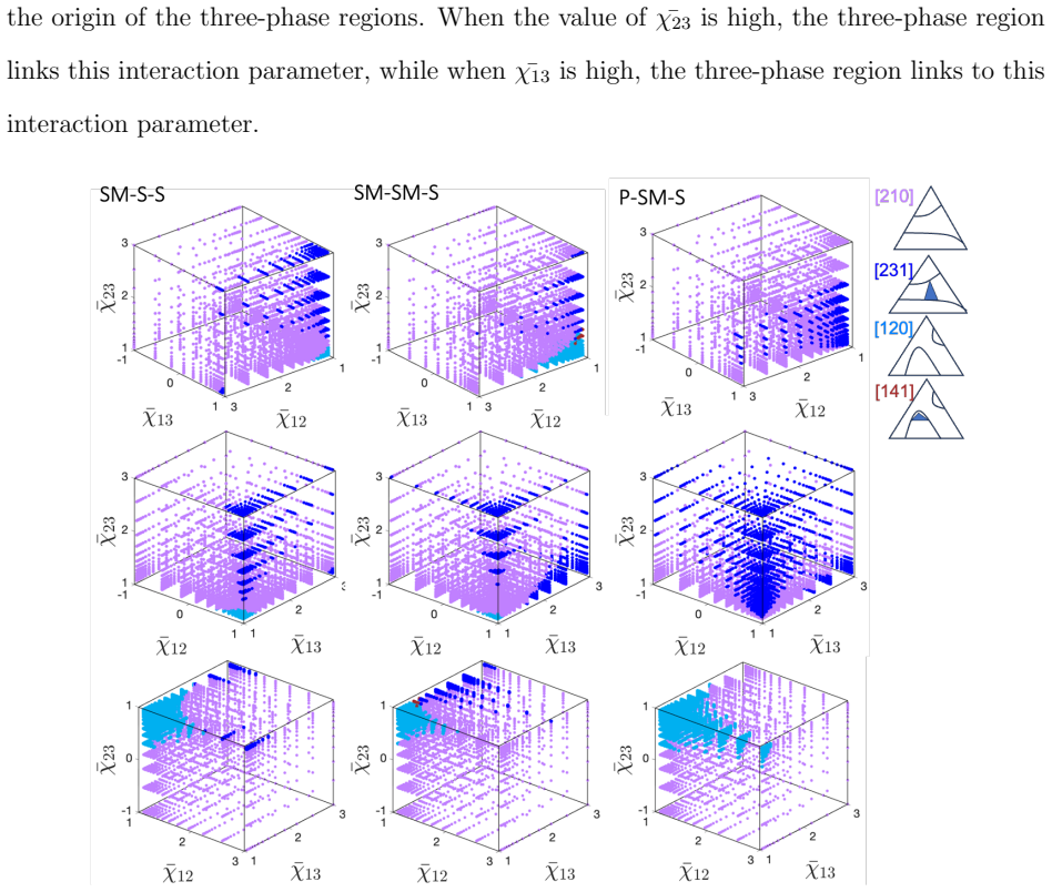
Within the standard lattice free-energy description of amorphous ternary blends, the paper establishes an octant rule: dividing the three-dimensional interaction-parameter space by the planes $\chi_{ij}=\chi^c_{ij}$ yields eight octants labelled by the number of immiscible binary pairs, and each octant has a dominant phase-diagram type that is the same for the three material classes studied. The full taxonomy lists 21 types, ordered by the number of one-, two-, and three-phase regions, with several types not reported before. The four types associated with 0, 1, 2, or 3 immiscible binary pairs are the most probable; the remaining types are confined to narrow slivers around the critical planes, and one type ([463]) appears exactly once in the 81,000-diagram library. The paper further argues that the miscibility depth of the common one-gap and two-gap diagrams is highly sensitive to interaction parameters near the critical planes but becomes less sensitive as molar size grows, and it validates the taxonomy against experimental diagrams, including a temperature-driven transition through three predicted types.
Load-bearing premise
The taxonomy rests on the numerical classification of phase regions on a 300-point grid, with a heuristic rule for judging which convex-hull triangles count as two- and three-phase regions; the authors acknowledge that this classification becomes ill-defined near critical interaction values and discard roughly 0.5% of the diagrams as incorrect.
Editorial extensions
If this is right
- In the three material systems studied, counting the binary pairs with $\chi_{ij}>\chi^c_{ij}$ determines the dominant phase-diagram type, so the first step in predicting a ternary diagram is comparing each interaction parameter with its pair-critical value.
- Rare types such as [130], [151], [241], and [463] occur almost exclusively near the critical planes, so routine material screening can treat them as low-probability events unless the parameters are deliberately tuned to that narrow window.
- For one-immiscible-pair systems the miscibility depth spans roughly two orders of magnitude (about 0.018 to 0.96 in the polymer case), while two-immiscible-pair systems show a compressed depth range and therefore less tunability through interaction-parameter choice.
- An experimental polymer system shifting through predicted types [151], [241], and [331] as temperature changes is reproduced by the model, indicating that the taxonomy captures real parameter-space trajectories, not just static labels.
Reading between the lines
- We infer a practical reproducibility rule the paper leaves implicit: choose component pairs whose interaction parameters are comfortably away from their critical values; systems tuned near the critical planes will have phase-diagram classes that are exquisitely sensitive to small batch-to-batch variations.
- We infer that the octant rule should hold for other molar-size combinations, with the same dominant types but different widths for the rare-type windows; scanning molar-size ratios continuously would turn the taxonomy into a quantitative design chart.
- A testable extension suggested by the method: applying the same high-throughput classification to quaternary blends should find that the number of immiscible binary pairs remains the first-order classifier, though the count of possible types grows much faster.
Signed reviews
Editorial analysis
A structured set of objections, weighed in public.
Referee Report
Summary. This paper constructs >81,000 Flory-Huggins ternary phase diagrams for three representative molar-size classes (polymer–small molecule–solvent, small molecule–small molecule–solvent, small molecule–solvent–solvent), classifies them into 21 phase-diagram types using a convex-hull algorithm with connected-component counting, and maps the types onto octants of the three-dimensional interaction-parameter space. The central proposal is a first-order existence rule: the number of binary pairs with interaction parameter above its critical value determines the dominant phase-diagram type, with uncommon types confined to narrow near-critical windows. The paper also reports sensitivity of miscibility depth for selected types and compares simulated diagrams with several literature experimental phase diagrams.
Significance. If the classification is numerically robust, the paper provides a valuable systematic resource: a large library of ternary phase diagrams, a compact taxonomy, and simple design rules that are plausible and practically useful for solvent selection in organic thin-film processing. The explicit enumeration of rare types, including some not reported previously, is a genuine contribution. The experimental comparisons are useful as qualitative consistency checks for types [110], [210], [331], [151], and [241]. However, the load-bearing numerical classification of rare types is not supported by convergence or threshold-sensitivity analyses, and the experimental validation is partly circular because interaction parameters are adjusted within the octant constraints. These issues prevent the paper from being accepted in its current form.
major comments (3)
- [Method — Phase diagram construction] The identification of two-phase versus three-phase regions relies on a heuristic sorting of projected convex-hull triangles by 'two elongated edges' versus 'three elongated edges', with a length threshold tied to the grid spacing. The authors explicitly state that this sorting is 'slightly sensitive to the criteria chosen' and that near critical χ values 'the identification of the triangles is ill-defined and where grid refinement only partly helps', with about 0.5% of diagrams judged incorrect and excluded. This matters because the rare types that constitute the paper's novelty—[130], [141], [151], [162], [172], [193], [220], [241], [262], [283], [352], [373], and [463]—are reported precisely in the near-critical windows where the method is acknowledged to be unreliable, and [463] is based on a single diagram. No grid-convergence or threshold-sensitivity analysis is reported. I ask the authors to quantify how the three-digit keys change under grid refinement (e.g., 150, 300, 600 points per direction) and under variation of the triangle-length threshold, and to report confidence or stability measures for the type assignment, especially for the rare types.
- [Validation of the simulated phase diagrams] The experimental validation is not an independent test of the proposed existence rules. In SI-5, the modeling interaction parameters are chosen to respect the octant constraint, but they deviate substantially from the reported experimental values in several cases. For example, Table 5 uses χmod_13 = 0.58 where the experimental value is χexp_13 = 2.07, and Tables 7 and 9 list χmod values whose selection rule from the measured data is not stated. The comparisons therefore demonstrate that the observed phase-diagram types can be reproduced with some parameters in the appropriate octant, which is a much weaker claim than 'successful comparisons ... showcase the real-world relevance.' To support the predictive claim, the authors should include at least one system with independently measured interaction parameters and no octant-constrained tuning, or provide a clear a priori protocol for choosing χmod values within the octant.
- [Octant-based existence rules] The claim of universality over material systems is stronger than the evidence. Only three molar-size combinations are simulated, and the paper itself reports system-dependent differences: type [130] is not found for the P-SM-S system, and type [120] is only found for SM-S-S and SM-SM-S. The first-order rule 'number of immiscible pairs controls the dominant type' is essentially true by construction of the input parameter space, but the detailed type distributions and the location of rare-type windows are not universal across the studied systems. I recommend softening 'universal' to 'common across the studied size ratios' or explicitly mapping where the distributions differ and adding at least one additional size-ratio set to test the universality claim.
minor comments (4)
- [Results] The sentence 'The fraction decreases s as the interaction parameter decreases' contains a stray character 's' and should be corrected.
- [Method — Phase diagram construction] The typeset form of Eq. (2) appears to show the radicals without the reciprocal prefixes; it should read χc_ij = 1/2 (1/√Ni + 1/√Nj)^2. Please check the rendering.
- [Results — Identification and classification] Because [110-o] is counted as one of the 21 types, the label should be more distinct from [110] in the figure, especially since the paper analyzes it separately.
- [Data generation] The text refers to the three libraries as P-SM-S, SM-SM-S, and SM-S-S, but the Data generation subsection also mentions additional sets for P-S-S and S-S-S; please clarify whether those additional sets are included in the 81,000 diagrams or are separate.
Circularity Check
The 21-type taxonomy is largely self-contained, but the experimental validation is partly circular because interaction parameters are fitted after the fact to reproduce the observed phase diagrams.
-
fitted input called prediction
[Section 'Validation of the simulated phase diagrams on typical organic thin film material systems'; SI-5, 'PMMA/acetone/n-hexane phase diagram']
"Still, within this constraint, some freedom is given for the choice of the exact value of the interaction parameters to compensate for the simplicity of the free energy function (Eq. 1) as compared to the real behavior of experimental systems. ... Using this constraint, the PMMA/acetone/n-hexane phase diagram is calculated ... using the interaction parameter values shown in the second column of Table 5."
The validation claims to confirm the existence rules against experimental phase diagrams, but for the multi-gap cases the simulation input chi_mod is not obtained from the measured chi_exp by a forward procedure. It is selected after the fact within the octant constraint (same side of the critical chi) so that the computed diagram matches the observed one; for example, in Table 5 chi_exp_13 = 2.07 while chi_mod_13 = 0.58, both above chi_c_13 = 0.28. The resulting 'quantitative and qualitative match' is therefore partly by construction: the output (phase diagram type and shape) is used to choose the input, so the comparison does not independently confirm the octant rules. The 21-type library and octant maps do not depend on these fits, so the circularity is confined to the validation layer.
full rationale
The central derivation chain is self-contained: Eq. (1)-(2) define the Flory-Huggins free energy and binary critical interaction parameters; the convex-hull construction converts (chi, N) into phase diagrams; and the three-digit keys are counts of connected one-, two-, and three-phase regions. The octant-based existence rules are empirical summaries of the 81,000 simulations, not definitions, and they are nontrivial because exceptions exist (e.g., [131] in one-chi-greater-than-critical octants and [110-o] in the all-miscible octant). The paper's own numerical caveats -- sensitivity near critical values, ill-defined triangle identification, and exclusion of about 0.5% of diagrams -- are correctness risks, not circularity. Self-citations to the authors' previous phase-field and convex-hull papers are not load-bearing: the convex-hull method is standard and is also cited to independent sources. The only concrete circular element is the experimental validation, where chi_mod values are fitted within octant constraints to reproduce observed diagrams and then presented as successful comparisons; this raises the score but does not infect the taxonomy itself, which remains an independent computational result.
Assumptions & free parameters
free parameters (3)
- Representative molar sizes (N1,N2,N3) =
(245,5,1), (5,5,1), (5,1,1), plus small pre-selected sets
- Screened interaction parameter range and sampling density =
chi_c - 2 chi_c to chi_c + 2 chi_c, logarithmic near chi = chi_c planes
- Validation interaction parameters chi_mod =
PS/MCH/EGDA: chi12=2.15, chi13=0.567, chi23=0.7; PMMA/acetone/n-hexane: chi12=1.495, chi13=0.58, chi23=0.37
assumptions (5)
- domain assumption Flory-Huggins free energy with constant composition-independent interaction parameters
- standard math Convex hull of the discretized free energy surface identifies equilibrium phase regions
- standard math Binary critical interaction parameters are given by Eq. 2
- ad hoc to paper Logarithmic sampling near critical planes captures all relevant phase diagram types
- ad hoc to paper Connected-component counting gives a meaningful three-digit classification key
Cite this review
Pith. "Pith review of Taxonomy of amorphous ternary phase diagrams: the importance of interaction parameters." pith.science (2026). https://pith.science/paper/DIC5AGCI
@misc{pith2026250104478,
  author       = {Pith},
  title        = {Pith review of: Taxonomy of amorphous ternary phase diagrams: the importance of interaction parameters},
  year         = {2026},
  howpublished = {\url{https://pith.science/paper/DIC5AGCI}},
  note         = {Machine review of arXiv:2501.04478}
}
abstract
Understanding phase diagrams is essential for material selection and design, as they provide a comprehensive representation of the thermodynamics of mixtures. This work delivers a broad and systematic overview of possible ternary phase diagrams for amorphous systems representative of polymers, small organic molecules, and solvents. Thanks to computationally efficient methods, an unprecedented library of $>$80,000 ternary phase diagrams is generated based on a systematic screening of interaction parameters. Twenty-one phase diagram types, including unreported ones, are identified. They are classified according to simple rules related to the number of immiscible material pairs, of miscibility gaps, and of three-phase regions. They are mapped onto the three-dimensional interaction parameters space, providing a clear picture of their likelihood and existence conditions. Four well-known phase-diagram types with 0, 1, 2, or 3 immiscible pairs are found to be the most likely. The numerous uncommon phase diagrams are mostly observed within a small parameter window around the critical interaction parameter values. For the most common phase diagram types, we show that the size of the processability window becomes sensitive to interaction parameter variations close to critical values. The sensitivity decreases for materials with increasing molar size. Finally, successful comparisons of simulated and experimental phase diagrams showcase the real-world relevance of this theoretical analysis. The presented results lay a robust foundation for rational design of solution processing conditions and for blend morphology control. Immediate applications include organic thin films and the identification of green solvents for sustainable processing.
Figures


Figures from the paper (10 more)




Reference graph
Works this paper leans on
-
[151]
N1 = 5, N2 = 1, N3 = 1 χ12 = 1.3017, χ13 = 1.3017, χ23 = 2.2869
-
[241]
N1 = 5, N2 = 5, N3 = 1 χ12 = 0.4441, χ13 = 1.0996, χ23 = 1.6091
-
[331]
N1 = 1, N2 = 1, N3 = 1 χ12 = 2.1694, χ13 = 2.3734, χ23 = 3.8145
-
[463]
The values used for all studied material systems are summarized in Table 3
N1 = 5, N2 = 1, N3 = 1 χ12 = 1.6081, χ13 = 1.6081, χ23 = 2.2204 SI-5: Parameters used for the modeling of experimental phase diagrams For the different systems studied, the molar sizes Ni = vi v0 are calculated using the species molar volumes vi = Mi ρi , where Mi and ρi are the species molar mass and density available from literature data, respectively. ...
work page 1922
-
[110]
N1 = 5, N2 = 1, N3 = 1 χ12 = 2.2837, χ13 = 1.0472, χ23 = 1.8699
-
[210]
(bottom). SI-4: Parameters used for each type of phase diagram identified The following table gives the material parameters used to reproduce the different types of phase diagrams identified in the main text. The density is fixed to 1000 kg m−3 for all the materials. 37 Table 2: Material parameters to illustrate the different types of phase diagrams ident...
-
[130]
N1 = 5, N2 = 1, N3 = 1 χ12 = 1.3017, χ13 = 1.2427, χ23 = 2.2204
-
[141]
N1 = 5, N2 = 5, N3 = 1 χ12 = 0.4339, χ13 = 0.9949, χ23 = 1.4782
-
[162]
N1 = 1, N2 = 1, N3 = 245 χ12 = 1.999, χ13 = 1.0649, χ23 = 1.0649
-
[172]
N1 = 1, N2 = 1, N3 = 1 χ12 = 2.6, χ13 = 2.6, χ23 = 2.6
-
[193]
N1 = 1, N2 = 1, N3 = 1 χ12 = 2.65, χ13 = 2.65, χ23 = 2.65
-
[220]
N1 = 5, N2 = 1, N3 = 1 χ12 = 1.1626, χ13 = 2.2837, χ23 = 2.6324
-
[262]
N1 = 1, N2 = 1, N3 = 1 χ12 = 2.7, χ13 = 2.72, χ23 = 2.63
-
[283]
N1 = 1, N2 = 1, N3 = 1 χ12 = 2.7, χ13 = 2.7, χ23 = 2.65
-
[352]
N1 = 1, N2 = 1, N3 = 1 χ12 = 2.63, χ13 = 2.75, χ23 = 2.8
-
[373]
N1 = 1, N2 = 1, N3 = 1 χ12 = 2.67, χ13 = 2.7, χ23 = 2.65
-
[120]
N1 = 5, N2 = 1, N3 = 1 χ12 = 1.1974, χ13 = 0.8517, χ23 = 2.1694
work page 1974
Show all 23 references
-
[8]
N1 = 5, N2 = 5, N3 = 1 χ12 = 0.42, χ13 = 0.3172, χ23 = 1.3784
-
[12]
One of the interaction parameters is below its critical value ( χ13 < χc
and a selected range for the two remaining interaction parameters. One of the interaction parameters is below its critical value ( χ13 < χc
-
[13]
while the other is above the critical value ( χ23 > χc 23). As χ13 approaches its critical value and χ23 is slightly above the critical value (right bottom corner 34 of the figure), the two-phase region is significantly smaller than when χ13 is significantly lower (left bottom...
1974
-
[100]
N1 = 245, N2 = 5, N3 = 1 χ12 = 0.0121, χ13 = 0.0525, χ23 = 0.0971 [110 − o] N1 = 5, N2 = 1, N3 = 1 χ12 = 1.0472, χ13 = 0.9949, χ23 = 1.8699
-
[131]
N1 = 5, N2 = 1, N3 = 1 χ12 = 2.6565, χ13 = 0.897, χ23 = 1.8699
-
[231]
N1 = 5, N2 = 1, N3 = 1 χ12 = 1.1974, χ13 = 0.9791, χ23 = 3.8145
1974
Reviewed August 10, 2026 · model on record in the stance chip above.
Discussion (0). Continue with ORCID to comment.