Solver-in-the-loop training of deep learning closures for large-eddy simulation of turbulent premixed jet flames

Jonathan F. MacArt; Priyesh Kakka

Solver-in-the-loop training of deep learning closures for large-eddy simulation of turbulent premixed jet flames

T0 review · 4 major / 4 minor · reviewed 2026-08-01 · deepseek-v4-flash

Challenge this review Re-run · record.json Download PDF Read on arXiv ↗ Review JSON

Pith's one-line read A neural-network eddy-viscosity closure trained inside the LES solver reduces resolved-field errors by 25–50% and resolved Reynolds-stress and scalar-flux errors by over 60%, while generalizing across Damköhler numbers.

desk verdict A credible proof-of-concept for solver-embedded closure training in reacting LES, with claims running ahead of the evidence. read the letter →

arxiv 2607.17376 v2 pith:DIHI74BR submitted 2026-07-19 physics.flu-dyn physics.comp-ph

Priyesh Kakka , Jonathan F. MacArt This is my paper · ORCID

classification physics.flu-dynphysics.comp-ph

keywords large-eddysimulationpremixedcombustionturbulenceclosureneuralnetworkadjoint-basedoptimizationdifferentiableprogrammingDamköhlernumbergeneralizationsubgrid-scalemodeling

verification ladder T0 review T1 audit T2 compute T3 formal

The pith

A machine-rendered reading of the paper's core claim, the machinery that carries it, and where it could break.

The reading

The paper tries to establish that a deep-learning turbulence closure for large-eddy simulation of premixed flames can be trained directly inside the solver—through adjoint-based gradients that respect the governing equations—rather than on precomputed data. The best model, a small neural network that augments the standard eddy-viscosity closure, is claimed to cut primitive-variable errors by 25–50% and resolved Reynolds-stress and scalar-flux errors by more than 60% relative to a constant-coefficient baseline. Crucially, the paper claims the learned closure remains stable and accurate at Damköhler numbers it was not trained on, including both the nonreacting and strongly burning limits. If true, this would give combustion LES a route to closures that adapt to turbulence–flame interactions across regimes without retuning per case.

What carries the argument

The machinery is an augmented eddy-viscosity closure: the baseline Smagorinsky eddy viscosity is retained and a multilayer perceptron (four layers, 100 hidden units, GELU activations, about 35,000 parameters) adds a learned correction, with one output channel for momentum/species transport and one for heat flux. The network is evaluated pointwise using Galilean-invariant local gradients of density, velocity, internal energy, product mass fraction, and pressure, together with the baseline eddy viscosity, the chemical source term, and time. Because the network is embedded in the PDE residual, parameter gradients are obtained by integrating an adjoint equation backward over each optimization wi

What would settle it

Run the trained ME20-PRvv closure in a posteriori LES of a spatially developing premixed jet at a Damköhler number outside {0, 20,000, 35,000} and at a higher Reynolds number, comparing against filtered DNS or experimental data; if the reported 25–50% and 60% error reductions do not reproduce or the solver becomes unstable, the generalization claim is falsified.

Watch

Extended reading notes

Core claim

The central claim is that embedding an untrained neural network into the filtered LES equations and fitting it with adjoint-based gradients yields a closure that recovers both mean fields and resolved turbulence statistics in turbulent premixed jet flames across Damköhler-number regimes. The best model, trained with a primitive-variable objective augmented by the flame-normal resolved Reynolds stress (the PRvv variant), improves primitive-variable errors by 25–50% and resolved Reynolds-stress and scalar-flux errors by more than 60% relative to the Smagorinsky baseline, while staying stable at out-of-sample conditions. The paper also finds that a two-output augmented eddy-viscosity form gener

Load-bearing premise

The central claim rests on a single temporally evolving planar premixed jet with one-step chemistry and one fixed Smagorinsky baseline; if that configuration does not represent practical premixed burners, the reported margins and cross-Damköhler generalization may not carry over.

Editorial extensions

If this is right

Solver-embedded neural closures can replace or augment constant-coefficient eddy-viscosity models in reacting-flow LES without becoming unstable during deployment.
Including second-order statistics in the training objective is necessary: models trained only on primitive variables leave resolved Reynolds stresses worse than the baseline.
The two-output augmented eddy-viscosity formulation is more robust than a high-dimensional direct-closure formulation, which becomes unstable in reacting regimes.
Serial-window training, where the LES evolves continuously across windows, generalizes better than parallel-window training for long-horizon predictions.
The learned closure maintains accuracy at out-of-sample Damköhler numbers, including the nonreacting limit and the strongly burning thin-flame regime.

Reading between the lines

Editorial extensions of the paper, not claims the author makes directly.

Because the demonstration uses one temporally evolving planar jet with single-step chemistry, the same recipe would need validation on more complex geometries and fuels before it can be called broadly applicable; the paper's framing leaves that step implicit.
The success of a small pointwise network with gradient inputs suggests a path toward online adaptive closures that update as the flow regime changes, rather than offline per-case tuning.
The comparison against only one fixed-coefficient Smagorinsky baseline leaves open whether the reported margins would shrink against dynamic or otherwise more advanced subgrid closures; a head-to-head test would be a useful extension.
The unresolved reaction source is not modeled explicitly but is assumed to be absorbed by the learned species-transport closure, so accuracy may degrade in cases where filtered-chemistry error dominates—an implicit limitation worth testing directly.

Share X Bluesky LinkedIn Reddit HN

Signed reviews

No signed human review yet.

Editorial analysis

A structured set of objections, weighed in public.

Desk editor's note, referee report, and a circularity audit.

Desk Editor's Note

read the letter

Closure training inside the LES solver is the right direction. This is the first application of the solver-in-the-loop DPM approach to reacting LES, and the paper does a genuinely careful job of comparing closure forms, training strategies, and objective functions. The loss curves and component-wise tables make the in-sample improvements plausible, and the authors are candid that the direct-closure model is unstable and that the unresolved reaction source is left unmodeled. Those are real disclosures.

The stress-test note lands. The baseline is Smagorinsky with Cs=0.3, a high-dissipation choice for a planar jet; a dynamic or lower-Cs comparator could absorb a large chunk of the reported gains. All results come from one temporally evolving planar jet with single-step chemistry. The network receives absolute time t as an input, which lets it memorize the training window, and the Damköhler number is given explicitly, so 'generalization' is more a labeled interpolation test than an extrapolation test. Table 2 shows JP=-11% at Das=0 for the preferred model, so the abstract's unconditional '25-50%' phrasing is wrong. There is no UQ, no code or data release, and the loss weights are empirically tuned.

None of this sinks the paper as a proof-of-concept. The method is well explained, the serial-vs-parallel and objective-function comparisons are valuable for the community, and the authors are honest about failures. The main fix is to align claims with evidence: either test a second configuration and a stronger baseline, or qualify the broad-applicability language.

I'd send it to peer review, because it deserves referee time. I'd want the authors to address the baseline and the time input before publication. I'd also cite the training-methodology results if I worked in this area.

Referee Report

4 major / 4 minor

Summary. The paper presents a solver-in-the-loop (adjoint/DPM) training framework for neural-network subgrid-scale closures in LES of a temporally evolving planar turbulent premixed jet flame. The closure augments a Smagorinsky baseline with an MLP that predicts an eddy viscosity (and a variant that predicts SGS fluxes directly), with training by adjoint-based gradients matching filtered DNS data over optimization windows. Several objective functions (P, PRvv, PSF), training strategies (serial, parallel-window, parallel-data), and Damköhler-number training conditions are compared. The best model, ME20-PRvv, is reported to improve primitive-variable errors by 25–50% and resolved Reynolds stress and scalar-flux errors by more than 60% relative to the Smagorinsky baseline, including out-of-sample Damköhler-number cases.

Significance. If the quantitative claims hold, this is a useful methodological advance: it demonstrates that PDE-consistent, adjoint-trained neural closures can be extended from non-reacting LES and RANS to LES of premixed flames, and it systematically compares loss formulations and training strategies. The cost analysis and GPU implementation are practical strengths, and the component-wise tables provide more information than a single aggregate metric. However, the broad-applicability conclusion and the headline percentage improvements are not yet fully supported because all results come from a single configuration with a single, possibly weak, comparator and without uncertainty quantification. The core idea is credible and worth publishing after strengthening the evidence and re-scoping the claims.

major comments (4)

[Sec. 2, Eq. (7); Sec. 6] The only comparator is the constant-coefficient Smagorinsky model with Cs=0.3. This is a particularly dissipative baseline for jet/free-shear flows; standard dynamic or locally adjusted Smagorinsky coefficients are typically lower. Since the ME network is initialized as a small correction to this baseline and trained against filtered DNS, the reported 25–50% and >60% improvements may be dominated by removal of excess baseline dissipation rather than by a genuinely superior closure. The central 'broadly applicable framework' claim therefore requires comparison against a stronger baseline (e.g., dynamic Smagorinsky or a well-tuned constant-Cs model) and, ideally, an established reacting-flow SGS closure.
[Sec. 6, Table 2; Figs. 2–5] All results are single-realization point estimates from one temporally evolving planar jet over the short interval t = 14.985–16.425 (Sec. 2). No uncertainty quantification, multiple initial conditions, or repeated training runs are reported. Because the optimization and evaluation involve chaotic LES trajectories, the specific percentage improvements are not established as statistically robust. At minimum, the authors should report ensemble/seed sensitivity or otherwise justify that the reported improvements are not within run-to-run variability.
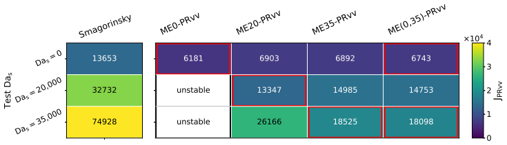
[Abstract and Table 2] The abstract claims the best model 'improves a posteriori errors in the LES primitive variables by 25–50%', but Table 2 reports JP = -11% for ME20-PRvv at Das = 0, 29% in-sample, and 41% at Das = 35,000. The claim is therefore not accurate as stated; it should be qualified by case and by loss component. This is a load-bearing inconsistency because it directly concerns the headline quantitative result.
[Secs. 2 and 6.3, Eq. (8)] The out-of-sample Damköhler-number tests are still within the same temporal planar-jet configuration, same Re/Ma, same filter width, and same single-step chemistry; only Das is varied. Moreover, the network receives the absolute time t as an input and is trained on the window t = 14.985–16.425, so it can in principle key onto the specific training interval. This limits the strength of the 'broadly applicable framework' conclusion. I recommend either adding a second configuration/initial condition (or retraining/testing on an interval not containing the training t window) or re-scoping the conclusions to the same configuration across Damköhler numbers.

minor comments (4)

[Sec. 6.3, Fig. 5] The vertical axis label 'JPRvv ×10^4' is ambiguous; specify whether this is the cumulative objective (13) or a single-window loss and give the normalization used for the percentage-improvement calculations.
[Sec. 7] CPU inference time is 642 s versus 100.5 s for Smagorinsky, a sixfold overhead, while GPU overhead is modest; the text should avoid implying the overhead is always modest without noting the CPU regime.
[Eq. (8)] The inclusion of Das and t as inputs is a design choice with potential generalization consequences. An ablation removing t, or at least a discussion of why the model does not simply memorize the training interval, would strengthen the out-of-sample interpretation.
[Sec. 6.1] The statement that the serial-window strategy is 'the most robust training configuration' is based on one reacting case. A caveat noting the limited evidence would be appropriate.

Circularity Check

0 steps flagged · score 0.0 of 10

No significant circularity: the central prediction step is a genuine held-out forward test against filtered DNS, and the load-bearing equations are derived in the paper rather than assumed from a self-citation.

full rationale

The paper's claimed derivation chain is: define the unclosed SGS terms (Eqs. 1–3), parameterize them with an augmented eddy-viscosity network (Eqs. 4–8), formulate a PDE-constrained adjoint optimization problem (Eqs. 10–18), train against filtered DNS in a series of assimilation windows, and then evaluate the trained closure at Damköhler numbers not used in training (Sec. 6.3). The out-of-sample evaluations at Das = 0 and Das = 35,000 for a model trained at Das = 20,000 are genuine forward tests: the fDNS targets at those conditions are never used in computing gradients, and the network must produce stable, accurate LES fields from its own closure. The inclusion of Das and t as network inputs is a modeling choice that may weaken the generality claim, but it does not make the prediction equal to the target by construction. The self-citations to the authors' own DPM framework [11–16] establish the methodology and supply the DNS configuration, but the paper re-derives the adjoint equations and the central quantitative comparison is to independently evolved Smagorinsky-baseline LES, not to the cited results. The weak constant-Cs baseline and single-planar-jet configuration are correctness/generalizability risks, not circularity; likewise, Table 2 shows JP = −11% at Das = 0 for the favored model, which contradicts the unqualified abstract claim but is an internal inconsistency rather than a circular reduction.

Assumptions & free parameters 7 free parameters · 6 assumptions · 0 invented entities

The central claim rests on a learned neural closure (fitted NN weights) plus several hand-chosen modeling constants and hyperparameters (Cs, Prt/Sct, loss weights, Nop, output scaling). No new physical entities are introduced; the closure is a functional mapping trained on filtered DNS data.

free parameters (7)

Neural network weights θ (ME) = 35,102 parameters
Fitted by adjoint-based optimization to filtered DNS targets; the central learned object (Sec. 3).
Neural network weights θ (DC) = 37,415 parameters
Direct-closure variant with 15 outputs; trained but less stable (Sec. 3).
ME output scaling factor = 1e-5
Multiplies NN outputs at initialization to keep forward LES stable (Sec. 3).
Smagorinsky coefficient Cs = 0.3
Baseline eddy-viscosity coefficient chosen for stable predictions; all improvements are measured against this baseline (Sec. 2.1, Eq. 7).
Turbulent Prandtl/Schmidt numbers = Prt=0.9, Sct=0.65
Fixed constants from earlier literature used in the gradient-diffusion closures (Sec. 2.1, Eqs. 5-6).
Objective weighting vectors SP, SR, SF = e.g., (1,1,1,1,0.083,1), (10^4,...,5e3), (100,100,100)
Empirically tuned to balance primitive and second-order losses (Sec. 4.1).
Optimization window length Nop = 60 steps
Manually chosen compromise between enough eddy turnover and adjoint divergence (Sec. 5).

assumptions (6)

domain assumption Favre-filtered compressible Navier-Stokes with single-step global chemistry govern the flow.
Basis of the DNS and LES equations; single-step chemistry isolates turbulent transport (Sec. 2).
domain assumption Boussinesq eddy-viscosity and gradient-diffusion forms are an adequate closure structure; only μt is augmented.
The NN predicts an augmented eddy viscosity; if the underlying ansatz is wrong, the model cannot recover true SGS physics (Sec. 2.1, Eqs. 4-6).
domain assumption The DNS dataset at three Damköhler numbers and one geometry spans the regimes of interest.
Training and generalization tests rely on Da_s ∈ {0, 20000, 35000} in a temporally evolving planar jet (Sec. 2).
ad hoc to paper Das and chemical source are valid regime-indicator inputs.
These inputs are included to help the network distinguish Damköhler regimes (Eq. 8); they make out-of-sample testing partly an interpolation on a labeled feature.
domain assumption Checkpointed adjoint with graph-breaking at each step gives usable parameter gradients.
Gradients are computed using stored states and algorithmic differentiation; this is an approximation to full backpropagation (Sec. 4, Eq. 18).
domain assumption Statistical homogeneity in streamwise/spanwise directions justifies Reynolds averaging over these directions.
Statistics Rij and FYP,j are defined via homogeneous-direction averages (Sec. 4.1).

how reviews work

0 comments

Cite this review

Pith. "Pith review of Solver-in-the-loop training of deep learning closures for large-eddy simulation of turbulent premixed jet flames." pith.science (2026). https://pith.science/paper/DIHI74BR

@misc{pith2026260717376,
  author       = {Pith},
  title        = {Pith review of: Solver-in-the-loop training of deep learning closures for large-eddy simulation of turbulent premixed jet flames},
  year         = {2026},
  howpublished = {\url{https://pith.science/paper/DIHI74BR}},
  note         = {Machine review of arXiv:2607.17376}
}

read the original abstract

Large-eddy simulation (LES) turbulence models often fail to capture the effects of chemical heat release and the resulting modulation of turbulence in premixed flames, underscoring the need for a framework that remains accurate across a broad range of physical regimes. We develop an augmented eddy-viscosity closure, based on deep neural networks calibrated jointly with the LES solution using adjoint-based optimization and differentiable programming, ensuring consistency with the governing partial differential equations (PDEs). Several objective functions and training methods are examined, and each model is assessed for its capability to interpolate and extrapolate across a wide range of Damk\"ohler numbers. Relative to the Smagorinsky-model baseline, the best neural network model improves a posteriori errors in the LES primitive variables by 25-50% and in the resolved Reynolds stress and scalar flux by more than 60%. Crucially, the model generalizes across Damk\"ohler number regimes, maintaining stability and accuracy even for out-of-sample conditions. These results demonstrate that PDE-consistent deep learning closures can recover both mean fields and resolved turbulence statistics in LES of turbulent premixed flames and can therefore provide a broadly applicable framework for turbulent combustion modeling.

Figures

Figures reproduced from arXiv: 2607.17376 by the authors.

**Figure 3.** Training-loss curves comparing ME20-PRvv, [PITH_FULL_IMAGE:figures/full_fig_p007_3.png] view at source ↗

**Figure 2.** Relative percentage improvements of ME model variants compared to the Smagorinsky baseline. Red bars denote in-sample results (Das = 20, 000); all other bars show out-of-sample performance. 0 100 200 300 400 Epoch 0.0 0.2 0.4 0.6 0.8 1.0 Relative MSE error ME20-PRvv ME20-PRvv-PW DC20-PRvv [PITH_FULL_IMAGE:figures/full_fig_p007_2.png] view at source ↗

Figures from the paper (2 more)

**Figure 4.** Figure 4: Component-wise validation losses for ME20-P, ME20-PRvv and ME20-PSF at [PITH_FULL_IMAGE:figures/full_fig_p009_4.png]

**Figure 5.** Figure 5: Performance of ME-PRvv models trained at different Damköhler numbers and evaluated at [PITH_FULL_IMAGE:figures/full_fig_p010_5.png]

Discussion (0). Continue with ORCID to comment.

Pith tools

Reviewed August 1, 2026 · model on record in the stance chip above.