REVIEW 4 major objections 6 minor 30 references
On identifiability and consistency of the nugget in Gaussian spatial process models
T0 review · 4 major / 6 minor · reviewed 2026-08-14 · deepseek-v4-flash
Pith's one-line read In Gaussian spatial models with a nugget, the nugget variance and the product σ²φ^{2ν} are identifiable and consistently estimable under in-fill asymptotics, while σ² and φ alone are not.
desk verdict Important identifiability result for the nugget, and clearly stated conditional consistency/CLT results, but the abstract oversells the theorems by hiding unproved spectral assumptions. read the letter →
The pith
A machine-rendered reading of the paper's core claim, the machinery that carries it, and where it could break.
The reading
What carries the argument
The engine is the eigendecomposition of the $n\times n$ observation covariance matrix $V_n = \tau^2 I_n + K_n$, where $K_n$ is the Matérn covariance matrix. The negative log-likelihood is written in the eigenbasis, and consistency follows from almost-sure convergence of weighted averages of iid $\chi^2_1$ variables; asymptotic normality follows from a Lindeberg central limit theorem for the same weighted sums. The analytic input that fixes the rates is a spectral law for the Matérn covariance matrix: on a regular grid its eigenvalues decay like $n i^{-2\nu/d - 1}$, with Assumption 1 supplying the lower bound and Assumption 2 the exact constant. This decay produces the normalization $n^{1/(2+4\nu/d)}$ in the CLT for the microergodic parameter. Identifiability is handled separately, by Gaussian-measure equivalence: for $d \le 3$, two measures agree exactly when $\tau^2$ and $\kappa = \sigma^2\varphi^{2\nu}$ agree, so only these two composite quantities can be recovered from dense sampling in a bounded domain.
What would settle it
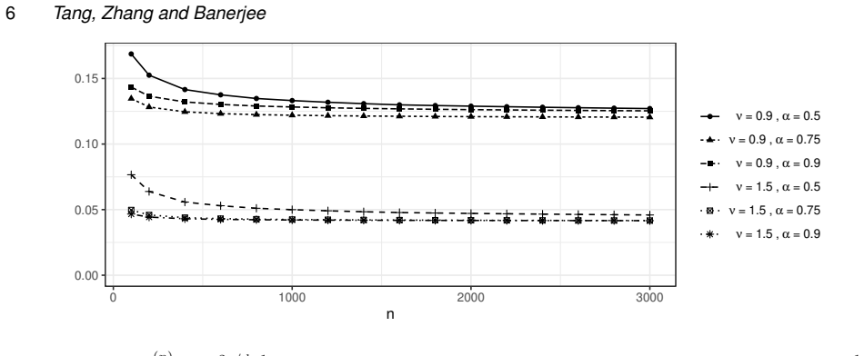
Take a Matérn covariance matrix on the regular grid in $d=2$ with, say, $\nu = 0.9$, and compute the scaled eigenvalues $\lambda_i^{(n)}/(n i^{-2\nu/d - 1})$ for $i = n^{\alpha}$ with $0 < \alpha < 1$ as $n$ grows. If for any such sequence the scaled eigenvalues tend to $0$ instead of to a positive constant, then Assumption 2 fails and the asymptotic normality of $\hat\sigma^2_n\varphi_1^{2\nu}$ is not supported by this paper's proof.
Extended reading notes
Core claim
For dimension $d \le 3$ and fixed smoothness $\nu > 0$, two Gaussian measures generated by the Matérn covariogram with nugget are equivalent if and only if they share the nugget $\tau^2$ and the microergodic combination $\kappa = \sigma^2\varphi^{2\nu}$; distinct nugget values yield orthogonal measures (Theorem 1). As a consequence, the maximum likelihood estimators $\hat\tau^2_n$ and $\hat\sigma^2_n\varphi_1^{2\nu}$ are strongly consistent (Theorem 4), and on a regular grid they satisfy the central limit theorems $\sqrt{n}(\hat\tau^2_n - \tau^2_0) \to N(0,\, 2\tau_0^4 c_2/c_1^2)$ and $n^{1/(2+4\nu/d)}(\hat\sigma^2_n\varphi_1^{2\nu} - \kappa_0) \to N(0,\, 2\varphi_1^{4\nu}/c_3)$ (Theorem 5). The rate for the microergodic parameter is slower than the $\sqrt{n}$ rate available without a nugget and reduces to the known $n^{1/4}$ rate for Ornstein–Uhlenbeck processes with measurement error when $\nu = 1/2$, $d = 1$.
Load-bearing premise
Everything about rates and normality rests on an unproven spectral assumption: on a regular grid the eigenvalues of the Matérn covariance matrix are bounded below by a positive constant times $n i^{-2\nu/d-1}$, and in fact converge to a fixed positive constant after this scaling; the paper offers heuristic and numerical support and says rigorous proofs are future work.
Editorial extensions
If this is right
- For $d \le 3$, dense sampling inside a bounded domain pins down the nugget $\tau^2$ and the product $\sigma^2\varphi^{2\nu}$, but never the partial sill or spatial scale separately.
- The nugget MLE converges at the standard $\sqrt{n}$ rate, while the microergodic parameter MLE converges at the slower $n^{1/(2+4\nu/d)}$ rate; for smooth processes and higher dimensions this is substantially slower.
- The underlying smooth spatial process can be consistently interpolated at unobserved locations even with a nugget, although predictions of the noisy observations carry irreducible error at least $\tau^2$.
- Prediction is asymptotically efficient only when the fitted model has the same $\tau^2$ and the same $\kappa$ as the generating model; the paper's simulations indicate this persists when $\varphi$ is estimated rather than fixed.
Reading between the lines
- If the spectral conjecture is proved, the same $n^{1/(2+4\nu/d)}$ rate should transfer to any stationary covariance whose spectral density decays like $u^{-2\nu-d}$, so the result likely extends beyond Matérn kernels.
- For Bayesian geostatistics, non-identifiability of $\sigma^2$ and $\varphi$ implies their posteriors keep following the prior even as $n$ grows, while $\tau^2$ and $\kappa$ posteriors concentrate; the authors gesture at this and it is a direct practical corollary.
- A natural stress test is to run the same estimation on irregular or clustered designs; if the eigenvalue lower bound only holds for regular grids, the consistency theorem may fail for designs with large gaps.
Signed reviews
Editorial analysis
A structured set of objections, weighed in public.
Referee Report
Summary. The paper studies fixed-domain (in-fill) asymptotics for a Gaussian process with Matérn covariance plus an additive nugget. Theorem 1 characterizes identifiability: Gaussian measures with different nuggets are orthogonal, and with equal nuggets they are equivalent in dimension d ≤ 3 exactly when the microergodic parameter κ = σ²φ^{2ν} matches, while for d ≥ 5 equivalence requires both σ² and φ to match. Corollary 1 concludes that σ² and φ are not consistently estimable when d ≤ 3. The paper then studies maximum likelihood estimation with φ fixed. An upper bound on the eigenvalues of the Matérn covariance matrix is proved in Corollary 2, but matching lower bounds are imposed as Assumption 1, and a stronger regular-grid limit is imposed as Assumption 2. Under these assumptions, Theorem 4 gives almost sure consistency of the nugget estimator τ̂² and of σ̂²φ₁^{2ν}, and Theorem 5 gives √n asymptotic normality for τ̂² and n^{1/(2+4ν/d)} asymptotic normality for the microergodic parameter. Simulations in d = 2 illustrate the likelihood geometry, the finite-sample behavior of the estimators, and prediction mean squared error.
Significance. If fully established, the results would fill a real gap in fixed-domain asymptotics: previous work largely excluded the nugget, and the paper identifies the different rates for the nugget (√n) and the microergodic parameter (n^{1/(2+4ν/d)}). Theorem 1 is a clean and useful identifiability result built on prior equivalence theorems of Zhang, Anderes, and Stein. Corollary 2, the eigenvalue upper bound, is a genuine technical contribution, and the paper ships reproducible simulation code. However, the central asymptotic claims are conditional on Assumptions 1 and 2, which are not proved; the paper itself states in the Discussion that rigorous proofs are future research. Because Lemma 2 and hence Theorems 4 and 5 depend directly on these assumptions, the advertised consistency results are not yet established unconditionally.
major comments (4)
- [§2.2.1, Assumptions 1–2; Theorems 4–5] The central consistency and CLT claims rest on Assumptions 1 and 2, whose lower-bound parts are not proved. Corollary 2 establishes only the upper bound λ_i^(n) ≤ C n i^{-2ν/d-1}. The text explicitly concedes that the regime i ≍ n^α with 0 < α < 1 is open, and Section 4 states that rigorous proofs of Assumptions 1 and 2 'will constitute future research.' Since Lemma 2(2)–(3) is exactly Assumptions 1 and 2, and since Theorem 4 and Theorem 5 are derived from that lemma, the consistency of σ̂²φ₁^{2ν} and the CLTs (16)–(17) collapse if the lower bound fails. The abstract presents the consistency results as established without this qualification, so the manuscript must either prove the assumptions or prominently reformulate the main claims as conditional on them.
- [§2.2.1, Assumption 2 and Lemma 2(3)] Assumption 2 states λ_i^(n)/(n i^{-2ν/d-1}) → A 'as n,i→∞' without specifying the joint mode of convergence. Lemma 2(3) and Theorem 5 then require convergence of the sums n^{-1}Σ(a⁰_ni)², n^{-1}Σ(a⁰_ni)⁴, and n^{-1/(1+2ν/d)}Σ(b⁰_ni)² in (15). Pointwise convergence along arbitrary sequences with n,i → ∞ does not by itself imply convergence of these Cesàro averages over i = 1,...,n. A uniform or dominated-convergence argument over the full range of i is needed; as written, the existence of the constants c₁, c₂, c₃ is not rigorously guaranteed. Since the proof of Lemma 2 is said to be 'elementary calculus' but is omitted, this gap is load-bearing for Theorem 5.
- [§2.2.2, Theorem 4 proof, Eq. (12)] The proof of consistency of τ̂² differentiates the likelihood to obtain Eq. (12), so the argument applies only to interior stationary points of the likelihood. However, Theorem 4 and the definition in (6) concern the global minimizer over the compact set D = [a,b] × [c,d]. No argument is given that the global argmin is eventually interior, nor is the boundary case handled separately. The theorem statement therefore overclaims relative to what the proof actually establishes; the paper's own introductory remark in Section 2.2 that the results concern 'stationary points' suggests this mismatch should be resolved explicitly.
- [§2.2.2, Theorem 4 proof, weighted averages after Eq. (12)] The proof asserts almost sure limits such as Σ W_i² a_ni² / Σ a_ni² → 1 by invoking Etemadi (2006, Theorem 1). But the weights a_ni = 1/(τ̂_n² + σ̂_n² λ_i) are random and depend on all W_i through the maximum likelihood estimators. The cited weighted strong law of large numbers does not directly apply as stated to weights that are functions of the same observations. The proof needs a conditioning or uniform-in-parameter argument, or a different martingale/adaptivity argument, before these weighted averages can be used to derive τ̂_n² → τ₀². This is a load-bearing step in the consistency proof.
minor comments (6)
- [§2.2, notation for λ_i] The definition of K_n includes σ² through K_w(·; σ², φ, ν), but the MLE algebra in (11)–(14) and Lemma 2 treats λ_i as eigenvalues of the correlation matrix, since V_n has eigenvalues τ² + σ² λ_i. Please define λ_i precisely (for example, as eigenvalues of the correlation matrix with unit variance) to remove this ambiguity.
- [§2.2.3, Theorem 5] The statement that the asymptotic normality 'holds for any compact set S ⊂ R^d' is not proved; either provide the argument or restrict the theorem to S = [0,1]^d.
- [§3.2, Table 3] In Table 3, the first row for τ₀² = 0.8 has the entries for n and φ₀ transposed: it reads '0.800 400 19.972' where the column order elsewhere is τ₀², φ₀, n.
- [§3.2, text before Tables 1–4] The sentence 'Table 4–4 list percentiles...' should read 'Tables 1–4 list...'.
- [§2.2, Eq. (5)] The quantity in (5) is called the 'rescaled' negative log-likelihood, but no rescaling by n is exhibited; clarify what the rescaling is or drop the word.
- [§3.3, profile likelihood (26)] In the profile likelihood expression, the matrix ρ(φ) and the profiling step over σ² should be defined explicitly, and the compact range over which φ and η are optimized should be stated.
Circularity Check
No circularity: results are conditional on unproved spectral assumptions, but the derivation does not reduce to its own inputs.
full rationale
The paper's derivation chain is self-contained in the sense required by the circularity audit. Theorem 1 (identifiability) is built on external measure-equivalence results (Stein 1999, Zhang 2004, Anderes 2010), none of which are authored by the present authors. Theorems 4 and 5 establish consistency and asymptotic normality of the MLE for the nugget and the microergodic parameter, using Assumptions 1 and 2 on the eigenvalue decay of the Matérn covariance matrix. These assumptions concern spectral properties of the covariance kernel, not the parameters being estimated, and the limits defining c1, c2, c3 in Lemma 2(3) and Theorem 5 are taken as assumptions rather than fitted quantities. The proofs do not rename a fitted parameter as a prediction; the MLE is the object of study, and the theorems characterize its behavior under the stated spectral hypotheses. The paper is transparent that Assumptions 1 and 2 are unproved: the Discussion states 'their rigorous proofs will constitute future research.' This makes the main theorems conditional on an external (presently conjectural) mathematical fact, which is a genuine limitation for the strength of the claims, but it is not circularity. There is no self-citation that carries a load-bearing step, no uniqueness theorem imported from the authors' own prior work, and no ansatz smuggled in via citation. The claims that are unchecked are assumptions about eigenvalues, not restatements of the estimation target. The paper even notes in Section 2.2.2 that the consistency of the nugget holds without Assumption 1, and the simulation studies are externally benchmarked against known results (Ornstein-Uhlenbeck cases). Accordingly, the honest finding is no significant circularity; the score is 0.
Assumptions & free parameters
assumptions (6)
- ad hoc to paper Assumption 1: there exists c > 0 such that the Matérn covariance matrix eigenvalues satisfy λ_i^{(n)} ≥ c n i^{-2ν/d-1} for all i = 1,...,n (lower spectral bound).
- ad hoc to paper Assumption 2: for the regular grid, λ_i^{(n)}/(n i^{-2ν/d-1}) → A > 0 as n, i → ∞.
- domain assumption Filling distance ~ n^{-1/d} and minimal separation ~ n^{-1/d} for sampled locations.
- domain assumption Smoothness parameter ν > 0 is known.
- standard math Parameter space for (τ², σ²) is compact D = [a,b] × [c,d] with 0 < a < b, 0 < c < d.
- standard math Gaussian measure equivalence/orthogonality results from Zhang (2004) and Anderes (2010) for the no-nugget Matérn model.
Cite this review
Pith. "Pith review of On identifiability and consistency of the nugget in Gaussian spatial process models." pith.science (2026). https://pith.science/paper/DK7N6TIH
@misc{pith2026190805726,
  author       = {Pith},
  title        = {Pith review of: On identifiability and consistency of the nugget in Gaussian spatial process models},
  year         = {2026},
  howpublished = {\url{https://pith.science/paper/DK7N6TIH}},
  note         = {Machine review of arXiv:1908.05726}
}
read the original abstract
Spatial process models popular in geostatistics often represent the observed data as the sum of a smooth underlying process and white noise. The variation in the white noise is attributed to measurement error, or micro-scale variability, and is called the "nugget". We formally establish results on the identifiability and consistency of the nugget in spatial models based upon the Gaussian process within the framework of in-fill asymptotics, i.e. the sample size increases within a sampling domain that is bounded. Our work extends results in fixed domain asymptotics for spatial models without the nugget. More specifically, we establish the identifiability of parameters in the Mat\'ern covariance function and the consistency of their maximum likelihood estimators in the presence of discontinuities due to the nugget. We also present simulation studies to demonstrate the role of the identifiable quantities in spatial interpolation.
Figures


Figures from the paper (1 more)

Reference graph
Works this paper leans on
- [1]
-
[2]
Interpolation of S patial D ata: S ome T heory for K riging
Stein ML. Interpolation of S patial D ata: S ome T heory for K riging. Springer-Verlag; 1999
work page 1999
-
[3]
Towards reconciling two asymptotic frameworks in spatial statistics
Zhang H, Zimmerman DL. Towards reconciling two asymptotic frameworks in spatial statistics. Biometrika 2005;92(4):921--936
work page 2005
-
[4]
Inconsistent estimation and asymptotically equal interpolations in model-based geostatistics
Zhang H. Inconsistent estimation and asymptotically equal interpolations in model-based geostatistics. Journal of the American Statistical Association 2004;99(465):250--261
work page 2004
-
[5]
Fixed-domain asymptotic properties of tapered maximum likelihood estimators
Du J, Zhang H, Mandrekar VS. Fixed-domain asymptotic properties of tapered maximum likelihood estimators. The Annals of Statistics 2009;37(6A):3330--3361
work page 2009
-
[6]
The role of the range parameter for estimation and prediction in geostatistics
Kaufman CG, Shaby BA. The role of the range parameter for estimation and prediction in geostatistics. Biometrika 2013;100(2):473--484
work page 2013
-
[7]
Bevilacqua M, Faouzi T, Furrer R, Porcu E. Estimation and prediction using generalized W endland covariance functions under fixed domain asymptotics. Ann Statist 2019;47(2):828--856
work page 2019
-
[8]
Ma P, Bhadra A. Kriging: B eyond M at\'ern. arXiv preprint arXiv:191105865 2019
work page 2019
Show all 30 references
-
[9]
Infill asymptotics for a stochastic process model with measurement error
Chen HS, Simpson DG, Ying Z. Infill asymptotics for a stochastic process model with measurement error. Statistica Sinica 2000;p. 141--156
2000
-
[10]
Handbook of M athematical F unctions: with F ormulas, G raphs, and M athematical T ables
Abramowitz M, Stegun A. Handbook of M athematical F unctions: with F ormulas, G raphs, and M athematical T ables. Dover; 1965
1965
-
[11]
Asymptotics and computation for spatial statistics
Zhang H. Asymptotics and computation for spatial statistics. In: Advances and Challenges in Space-time Modelling of Natural Events Springer; 2012.p. 239--252
2012
-
[12]
On the consistent separation of scale and variance for G aussian random fields
Anderes E. On the consistent separation of scale and variance for G aussian random fields. The Annals of Statistics 2010;38(2):870--893
2010
-
[13]
Approximation beats concentration? A n approximation view on inference with smooth radial kernels
Belkin M. Approximation beats concentration? A n approximation view on inference with smooth radial kernels. In: Conference On Learning Theory, COLT 2018; 2018. p. 1348--1361
2018
-
[14]
Approximation of eigenfunctions in kernel-based spaces
Santin G, Schaback R. Approximation of eigenfunctions in kernel-based spaces. Advances in Computational Mathematics 2016;42(4):973--993
2016
-
[15]
Error estimates and condition numbers for radial basis function interpolation
Schaback R. Error estimates and condition numbers for radial basis function interpolation. Advances in Computational Mathematics 1995;3(3):251--264
1995
-
[16]
Asymptotic estimates of the n-widths in H ilbert space
Jerome JW. Asymptotic estimates of the n-widths in H ilbert space. Proceedings of the American Mathematical Society 1972;33(2):367--372
1972
-
[17]
Convergence of weighted averages of random variables revisited
Etemadi N. Convergence of weighted averages of random variables revisited. Proceedings of the American Mathematical Society 2006;134(9):2739--2744
2006
-
[18]
Asymptotic properties of a maximum likelihood estimator with data from a G aussian process
Ying Z. Asymptotic properties of a maximum likelihood estimator with data from a G aussian process. Journal of Multivariate Analysis 1991;36(2):280--296
1991
-
[19]
Asymptotically efficient prediction of a random field with a misspecified covariance function
Stein ML. Asymptotically efficient prediction of a random field with a misspecified covariance function. The Annals of Statistics 1988;p. 55--63
1988
-
[20]
A simple condition for asymptotic optimality of linear predictions of random fields
Stein ML. A simple condition for asymptotic optimality of linear predictions of random fields. Statistics & Probability Letters 1993;17(5):399--404
1993
-
[21]
Practical methods of optimization
Fletcher R. Practical methods of optimization. John Wiley & Sons; 2013
2013
-
[22]
A comparison of kriging with nonparametric regression methods
Yakowitz S, Szidarovszky F. A comparison of kriging with nonparametric regression methods. Journal of Multivariate Analysis 1985;16(1):21--53
1985
-
[23]
On fixed-domain asymptotics and covariance tapering in Gaussian random field models
Wang D, Loh WL, et al. On fixed-domain asymptotics and covariance tapering in Gaussian random field models. Electronic Journal of Statistics 2011;5:238--269
2011
-
[24]
Estimation and Model Identification for Continuous Spatial Processes
Vecchia AV. Estimation and Model Identification for Continuous Spatial Processes. Journal of the Royal Statistical society, Series B 1988;50:297--312
1988
-
[25]
@esa ( ) , n @biblabelnum##1 ##1
\@ifclassloaded aguplus natbib The aguplus class already includes natbib coding, so you should not add it explicitly Type <Return> for now, but then later remove the command natbib from the document \@ifclassloaded nlinproc natbib The nlinproc class already includes natbib cod...
-
[26]
@stdbsttrue NAT@ctr \@lbibitem[ NAT@ctr ] \@lbibitem[#1]#2 \@ifundefined b@#2\@extra@b@citeb @num @parse #2 [ @natanchorstart #2 \@biblabel @num @natanchorend] @ifcmd#1()()\@nil #2 @lbibitem\@undefined @lbibitem\@lbibitem \@lbibitem[#1]#2 @lbibitem[#1] #2 @ @@label #2 @stdbst ...
-
[27]
@open @close @open @close and [1] URL: #1 \@ifundefined chapter * \@mkboth \@ifundefined NAT@sectionbib * \@mkboth * \@mkboth\@gobbletwo \@ifclassloaded amsart * \@ifclassloaded amsbook * \@ifundefined bib@heading @heading NAT@ctr thebibliography [1] @ \@biblabel NAT@ctr \@bib...
-
[28]
, " * write output.state after.block = add.period write newline
ENTRY address author booktitle chapter edition editor howpublished institution journal key month note number organization pages publisher school series title type url volume year label extra.label sort.label short.list INTEGERS output.state before.all mid.sentence after.senten...
-
[29]
write newline
" write newline "" before.all 'output.state := FUNCTION n.dashify 't := "" t empty not t #1 #1 substring "-" = t #1 #2 substring "--" = not "--" * t #2 global.max substring 't := t #1 #1 substring "-" = "-" * t #2 global.max substring 't := while if t #1 #1 substring * t #2 gl...
-
[30]
write newline
" write newline "" before.all 'output.state := FUNCTION n.dashify 't := "" t empty not t #1 #1 substring "-" = t #1 #2 substring "--" = not "--" * t #2 global.max substring 't := t #1 #1 substring "-" = "-" * t #2 global.max substring 't := while if t #1 #1 substring * t #2 gl...
Reviewed August 14, 2026 · model on record in the stance chip above.
Discussion (0). Continue with ORCID to comment.