REVIEW 3 major objections 4 minor 37 references
Regularized Random Fourier Features and Finite Element Reconstruction for Operator Learning in Sobolev Space
T0 review · 3 major / 4 minor · reviewed 2026-08-03 · deepseek-v4-flash
Pith's one-line read Frequency-weighted Tikhonov regularization makes random Fourier feature matrices well-conditioned at N ~ m log m features, and RRFF-FEM then learns noisy PDE operators more accurately and faster than unregularized random features.
desk verdict A solid, incremental random-feature method for noisy operator learning; the main theorem's condition (6) appears violated in the tested regime, but the empirical claims and Student-t generalization are worth referee time. read the letter →
The pith
A machine-rendered reading of the paper's core claim, the machinery that carries it, and where it could break.
The reading
What carries the argument
The load-bearing object is the random feature matrix A∈C^{m×N} with entries exp(i⟨ω_k, x_j⟩). Its normalized Gram matrix (1/N)AA* concentrates around the kernel matrix whose entries are the Matérn characteristic function ϕ_ω(x_j−x_k) = E[exp(i⟨ω, x_j−x_k⟩)], the Fourier transform of the Student-t sampling density. Because this characteristic function is positive, decreasing in distance, and bounded by its value at the minimum spacing κ, standard row-sum bounds for Hermitian matrices control the deviation of the expected Gram matrix from the identity; a matrix concentration inequality then converts the per-entry bounds into the high-probability spectral concentration of Theorem 3.1. The secon
What would settle it
Compute the left-hand side of condition (6) with the experiment's parameters — take σ and ν from the parameter tables, κ equal to the smallest grid spacing, and m the number of output collocation points. In several reported settings σκ is small and the Matérn characteristic function is close to 1, so the product with m is much larger than η; checking whether the empirical spectral norm ‖(1/N)AA* − I_m‖₂ nevertheless stays below 2η with probability at least 1−δ would settle whether the concentration holds despite the unverified hypothesis.
Extended reading notes
Core claim
On the paper's own terms, the central claim is Theorem 3.1: with feature weights drawn from the multivariate Student's t density (scale σ, degrees of freedom ν), if N ≥ C η^{-2} m log(2m/δ) and the Matérn characteristic function evaluated at the minimum separation κ of the training points is at most η/m, then with probability at least 1−δ the normalized Gram matrix satisfies ‖(1/N)AA* − I_m‖₂ ≤ 2η. This concentration makes the least-squares system well conditioned and the pseudoinverse well defined, which the paper says yields estimation and generalization bounds. The method itself solves, for each output component, a regularized least squares problem whose penalty ∑‖ω_k‖_2^p |x_k|² suppress
Load-bearing premise
The main guarantee requires the kernel's value at the shortest distance between any two training points to be at most η/m; in the paper's experiments the frequency scale is so small that this value is near 1, so the theorem's hypotheses appear to be unmet in the very regime where the numerical gains are shown, and the stated estimation/generalization bounds are inherited from earlier work rather than proved.
Editorial extensions
If this is right
- With N ~ m log m features and the scale condition met, the feature matrix is spectrally concentrated around the identity, so the regularized least-squares problem is stable and the pseudoinverse is well defined.
- The frequency-weighted penalty suppresses high-frequency noise, which the experiments indicate lowers test error on all benchmark PDEs compared to the unregularized random feature model.
- Because RRFF-FEM's output is a finite element interpolant, the learned operator can be evaluated at arbitrary points of the output domain, not just the training grid.
- The experiments indicate that RRFF retains the speed advantage of random features, with training times below those reported for Matérn and RBF kernel methods on the same problems.
Reading between the lines
- A natural parameter-selection rule follows from condition (6): pick σ and ν so that the Matérn characteristic function at the grid spacing falls below η/m; tuning σ this way could bring the experiments into the regime where the theorem applies.
- Because ν=1 gives Cauchy and ν→∞ gives Gaussian weights, the Student-t family offers a one-parameter interpolation between heavy-tailed and light-tailed sampling, which could be matched to the regularity of a given PDE's solution operator.
- The frequency penalty ∑‖ω_k‖^p |x_k|² can be read as an RKHS Sobolev-norm penalty; this connection suggests a testable comparison against direct Sobolev-space kernel methods on the same noisy benchmarks.
- The FEM recovery map decouples the number of training samples from the output grid resolution; a competing implementation could replace it with learned recovery maps and measure how much of the reported gain comes from the interpolation step.
Editorial analysis
A structured set of objections, weighed in public.
Referee Report
Summary. The paper proposes a regularized random Fourier feature method (RRFF) and a finite-element variant (RRFF-FEM) for learning PDE solution operators from noisy data. Random feature weights are drawn from multivariate Student's t distributions, and a frequency-weighted Tikhonov term is added to the least-squares objective. The main theoretical result, Theorem 3.1, gives a high-probability bound on the deviation of the normalised random feature Gram matrix from the identity under conditions (5)–(6), and the paper states that this yields estimation and generalization bounds. Extensive experiments on advection, Burgers, Darcy, Helmholtz, Navier–Stokes, and structural mechanics benchmark problems compare RRFF/RRFF-FEM with unregularized RFF, kernel methods, and neural operators.
Significance. If the theoretical guarantee held in the parameter regime used in the experiments, the paper would be a useful contribution: it unifies and extends prior random-feature conditioning results to Student-t features, gives the advertised N = O(m log m) scaling, and the benchmark suite is unusually broad and accompanied by code. The proof of Theorem 3.1 appears internally consistent under its stated hypotheses. However, the main load-bearing condition is not verified and is implausible for the reported experimental parameters, and the estimation/generalization consequences are only asserted. The numerical study is substantial and the empirical improvements are interesting, but the advertised provable well-conditioning is not actually connected to the experiments in the present form.
major comments (3)
- [§3.2, Theorem 3.1, Eq. (6)] Condition (6) is load-bearing but never verified, and it is not satisfied by the reported experimental parameter values. Since φ(t) is the characteristic function of the feature distribution, φ(0)=1 and φ decreases with ∥t∥; therefore (6) requires the minimum separation κ among the rows of A — the training input functions, not the spatial grid — to be large enough that φ(κ) ≤ η/m. For the Gaussian case and the reported Darcy/Helmholtz scale σ=√2×10^{-5}, (6) reads exp(-σ²κ²/2) ≤ η/m, so for m=10^3–10^4 one needs κ of order 10^5; the discretized PDE input vectors have Euclidean norms of order 10–10^3, so this is not attainable. The paper never computes κ or checks (6). Even if κ could be chosen large, the very small η forced by (6) would make condition (5) require far more than the reported N. Consequently Theorem 3.1 does not apply in the regime where RRFF is tested, and the statement th
- [§3.2, final paragraph] The paper asserts that the concentration property can be used to derive estimation and generalization bounds 'similar to [18]', but no statement or proof is given. This is not a routine corollary: the estimator in (3) solves a regularized, frequency-weighted least-squares problem with Student-t features, whereas [18] analyzes unregularized minimum-norm interpolation with Cauchy features. The abstract and introduction advertise these guarantees, so the missing derivation is load-bearing. Either state the precise bounds and prove them, or explicitly limit the theoretical claim to the conditioning result.
- [§4.2–§4.3, Tables 7 and 10] The regularization parameter α is selected by minimizing the reported average relative test error ('we tested a range of values for α to find the optimal α such that the RRFF method minimizes the test error', Figures 8 and 12), and Tables 7 and 10 report the corresponding errors. This is a test-set leak: the reported 'test' errors no longer measure genuine generalization. The observed improvement of RRFF over RFF may therefore be inflated. Use a held-out validation split or nested cross-validation to choose α, and report test errors only for the final model.
minor comments (4)
- [§3, definition of ρ(ω)] The normalization factor appears to be σ π^{d/2} ν^{d/2} Γ(ν/2), but a d-dimensional scale parameter σ should give a factor σ^d π^{d/2} ν^{d/2} Γ(ν/2). Please correct the density or clarify the notation for σ.
- [§2 vs §3.2] The symbol m is overloaded: in Section 2 it denotes the output dimension, while in Assumption 1 and Theorem 3.1 it denotes the number of training samples. This makes the statement of condition (6) confusing and should be fixed by renaming one of the two quantities.
- [§2, Lipschitz assumption] The displayed Lipschitz condition contains a typo: ∥u2−u2∥ should presumably be ∥u1−u2∥.
- [§4.7, Table 7] The phrase 'consistently outperform' is stronger than the data support for Navier–Stokes with ν=2,3, where the reported differences are only 0.04–0.06 percentage points. Reporting standard deviations or confidence intervals over the 20 trials would help assess these differences.
Circularity Check
No significant circularity: Theorem 3.1 is independently proven from stated assumptions; only the generalization-bound corollary is imported from a same-group preprint.
-
self citation load bearing
[Section 1 (Contributions bullet 2) and end of Section 3]
"We show that if the complexity ratio N/m scales like log m, where N is the number of random features and m is the number of training samples, then the random feature matrix is well-conditioned with high probability. Estimation and generalization bounds follow from [18]. ... We can use the concentration property of the random feature matrix A∈C^{m×N} to derive estimation and generalization bounds similar to [18]."
The paper's advertised theoretical payoff—'which yields estimation and generalization guarantees'—is not derived in this paper. It is deferred to [18], an arXiv preprint by Liao, Needell, and Schaeffer, which shares the current author Hayden Schaeffer and is not reproduced or machine-checked here. No proof is given that the regularized Student-t estimator in (3) satisfies the assumptions or inherits the Cauchy-feature bounds of [18]. Thus the generalization-guarantee component of the central claim reduces to an unverified self-citation. This is partial and minor, because the well-conditioning theorem itself is proven independently through the Matérn characteristic function, Gershgorin, and Matrix Bernstein arguments.
full rationale
The main theoretical result, Theorem 3.1, is not circular: it is a genuine derivation from Assumption 1 and the explicit conditions (5)-(6). The proof identifies the Student-t characteristic function with the Matérn kernel, uses the minimum-separation assumption κ, and applies Gershgorin plus Matrix Bernstein. Condition (6) is an explicit sufficient condition on the kernel off-diagonal entries, not a fitted parameter, and the theorem does not claim it holds automatically. The experimental RRFF/RRFF-FEM results are evaluated on external benchmark PDEs from [24,7], so the reported improvements over RFF are not forced by construction. The main correctness caveat—that condition (6) appears not to be verified in the experimental regime, since σ√νκ is small and φ(κ)≈1—is an applicability gap, not a circularity. The only circularity-adjacent item is the import of estimation/generalization bounds from [18], a same-group preprint with no derivation supplied; this is a minor self-citation rather than a reduction of the central claim to its inputs. Overall score 2.
Assumptions & free parameters
free parameters (6)
- Feature scale σ =
0.001–0.2 (Tables 1–6)
- Regularization strength α =
10^-5–0.5 (Tables 1–6)
- Regularization exponent p =
2 or 4
- Number of random features N =
5,000–100,000
- Student-t degrees of freedom ν =
2, 3, ∞
- FEM mesh / grid size =
27–6,800 grid points
assumptions (6)
- domain assumption Training noise is i.i.d., isotropic Gaussian, with relative magnitude fixed per problem and test inputs also corrupted.
- domain assumption The target operator G is Lipschitz and each component f_j is Lipschitz.
- domain assumption Assumption 1: training points are separated by ||x_j − x_j'|| ≥ κ > 0 and feature weights follow a Student-t distribution.
- standard math Student-t random features generate a Matérn kernel whose RKHS equals the Sobolev space H^{(ν+d)/2}.
- domain assumption Estimation and generalization bounds from [18] apply to the regularized Student-t estimator.
- standard math Matrix Bernstein inequality, Gershgorin's theorem, Sobolev embedding, and Bessel function monotonicity are valid and applicable.
Cite this review
Pith. "Pith review of Regularized Random Fourier Features and Finite Element Reconstruction for Operator Learning in Sobolev Space." pith.science (2026). https://pith.science/paper/DR6JABGH
@misc{pith2026251217884,
  author       = {Pith},
  title        = {Pith review of: Regularized Random Fourier Features and Finite Element Reconstruction for Operator Learning in Sobolev Space},
  year         = {2026},
  howpublished = {\url{https://pith.science/paper/DR6JABGH}},
  note         = {Machine review of arXiv:2512.17884}
}
abstract
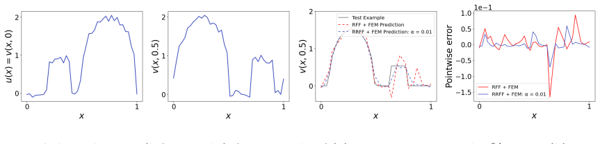
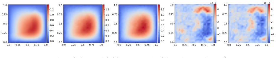
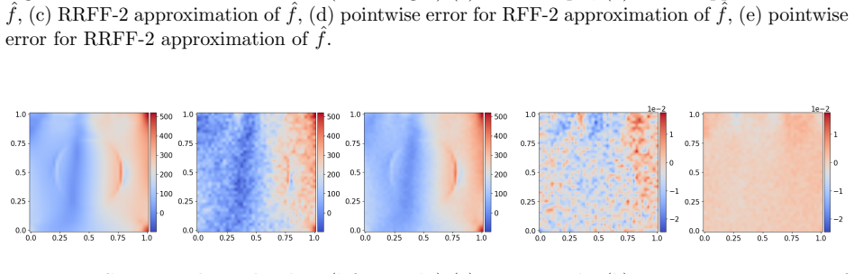
Operator learning is a data-driven approximation of mappings between infinite-dimensional function spaces, such as the solution operators of partial differential equations. Kernel-based operator learning can offer accurate, theoretically justified approximations that require less training than standard methods. However, they can become computationally prohibitive for large training sets and can be sensitive to noise. We propose a regularized random Fourier feature (RRFF) approach, coupled with a finite element reconstruction map (RRFF-FEM), for learning operators from noisy data. The method uses random features drawn from multivariate Student's $t$ distributions, together with frequency-weighted Tikhonov regularization that suppresses high-frequency noise. We establish high-probability bounds on the extreme singular values of the associated random feature matrix and show that when the number of features $N$ scales like $m \log m$ with the number of training samples $m$, the system is well-conditioned, which yields estimation and generalization guarantees. Detailed numerical experiments on benchmark PDE problems, including advection, Burgers', Darcy flow, Helmholtz, Navier-Stokes, and structural mechanics, demonstrate that RRFF and RRFF-FEM are robust to noise and achieve improved performance with reduced training time compared to the unregularized random feature model, while maintaining competitive accuracy relative to kernel and neural operator tests.
Figures


Figures from the paper (42 more)




Reference graph
Works this paper leans on
-
[18]
Cauchy random features for operator learning in Sobolev space.arXiv preprint arXiv:2503.00300, 2025
Chunyang Liao, Deanna Needell, and Hayden Schaeffer. Cauchy random features for operator learning in Sobolev space.arXiv preprint arXiv:2503.00300, 2025
arXiv 2025
-
[1]
Representation equivalent neural operators: A framework for alias-free operator learning
Francesca Bartolucci, Emmanuel de B’ezenac, Bogdan Raoni’c, Roberto Molinaro, Siddhartha Mishra, and Rima Alaifari. Representation equivalent neural operators: A framework for alias-free operator learning. InNeural Information Processing Systems, 2023
2023
-
[2]
Kernel methods are competitive for operator learning.Journal of Computational Physics, 2023
Pau Batlle, Matthieu Darcy, Bamdad Hosseini, and Houman Owhadi. Kernel methods are competitive for operator learning.Journal of Computational Physics, 2023
2023
-
[3]
Approximations of continuous functionals by neural networks with application to dynamic systems.IEEE Transactions on Neural networks, 4(6):910–918, 1993
Tianping Chen and Hong Chen. Approximations of continuous functionals by neural networks with application to dynamic systems.IEEE Transactions on Neural networks, 4(6):910–918, 1993
1993
-
[4]
Tianping Chen and Hong Chen. Universal approximation to nonlinear operators by neural networks with arbitrary activation functions and its application to dynamical systems.IEEE transactions on neural networks, 6(4):911–917, 1995
1995
-
[5]
Conditioning of random Fourier feature matrices: Dou- ble descent and generalization error.Information and Inference: A Journal of the IMA, 13(2):iaad054, 2024
Zhijun Chen and Hayden Schaeffer. Conditioning of random Fourier feature matrices: Dou- ble descent and generalization error.Information and Inference: A Journal of the IMA, 13(2):iaad054, 2024
2024
-
[6]
Concentration of random feature matrices in high-dimensions
Zhijun Chen, Hayden Schaeffer, and Rachel Ward. Concentration of random feature matrices in high-dimensions. InMathematical and Scientific Machine Learning, pages 287–302. PMLR, 2022
2022
-
[7]
de Hoop, Daniel Zhengyu Huang, Elizabeth Qian, and Andrew M
Maarten V. de Hoop, Daniel Zhengyu Huang, Elizabeth Qian, and Andrew M. Stuart. The cost-accuracy trade-off in operator learning with neural networks.Journal of Machine Learn- ing, 1(3):299–341, 2022
2022
Show all 37 references
-
[8]
Approximation rates of DeepONets for learning operators arising from advection-diffusion equations.Neural Networks, 153:411–426, 2022
Beichuan Deng, Yeonjong Shin, Lu Lu, Zhongqiang Zhang, and George Em Karniadakis. Approximation rates of DeepONets for learning operators arising from advection-diffusion equations.Neural Networks, 153:411–426, 2022
2022
-
[9]
Evans.Partial differential equations
Lawrence C. Evans.Partial differential equations. American Mathematical Society, Providence, R.I., 2010. 28
2010
-
[10]
Learning from non-random data in Hilbert spaces: An optimal recovery perspective.Sampling Theory, Signal Processing, and Data Analysis, 20, 2022
Simon Foucart, Chunyang Liao, Shahin Shahrampour, and Yinsong Wang. Learning from non-random data in Hilbert spaces: An optimal recovery perspective.Sampling Theory, Signal Processing, and Data Analysis, 20, 2022
2022
-
[11]
Gin, Daniel E
Craig R. Gin, Daniel E. Shea, Steven L. Brunton, and J. Nathan Kutz. DeepGreen: Deep learn- ing of Green’s functions for nonlinear boundary value problems.Scientific Reports, 11(1):21614, 2021
2021
-
[12]
Generalization bounds for sparse random feature expansions.Applied and Computational Harmonic Analysis, 62:310–330, 2023
Abolfazl Hashemi, Hayden Schaeffer, Robert Shi, Ufuk Topcu, Giang Tran, and Rachel Ward. Generalization bounds for sparse random feature expansions.Applied and Computational Harmonic Analysis, 62:310–330, 2023
2023
-
[13]
Huang, Kailai Xu, Charbel Farhat, and Eric Darve
Daniel Z. Huang, Kailai Xu, Charbel Farhat, and Eric Darve. Learning constitutive relations from indirect observations using deep neural networks.Journal of Computational Physics, 416:109491, 2020
2020
-
[14]
Bridging traditional and machine learning-based algorithms for solving PDEs: The random feature method.Journal of Machine Learning, 1(3):268–298, 2022
Chen Jingrun, Chi Xurong, E Weinan, and Yang Zhouwang. Bridging traditional and machine learning-based algorithms for solving PDEs: The random feature method.Journal of Machine Learning, 1(3):268–298, 2022
2022
-
[15]
Kovachki, Samuel Lanthaler, and Siddhartha Mishra
Nikola B. Kovachki, Samuel Lanthaler, and Siddhartha Mishra. On universal approximation and error bounds for Fourier neural operators.ArXiv, abs/2107.07562, 2021
2021 arXiv
-
[16]
Samuel Lanthaler and Nicholas H. Nelsen. Error bounds for learning with vector-valued random features. InProceedings of the 37th International Conference on Neural Information Processing Systems, NIPS ’23, Red Hook, NY, USA, 2023. Curran Associates Inc
2023
-
[17]
Fourier neural operator for parametric partial differential equations
Zongyi Li, Nikola Borislavov Kovachki, Kamyar Azizzadenesheli, Burigede Liu, Kaushik Bhat- tacharya, Andrew Stuart, and Anima Anandkumar. Fourier neural operator for parametric partial differential equations. InInternational Conference on Learning Representations, 2021
2021
-
[19]
Differentially private random feature model.arXiv preprint arXiv:2412.04785, 2024
Chunyang Liao, Deanna Needell, Hayden Schaeffer, and Alexander Xue. Differentially private random feature model.arXiv preprint arXiv:2412.04785, 2024
2024 arXiv
-
[20]
Generalization error guaranteed auto- encoder-based nonlinear model reduction for operator learning.Applied and Computational Harmonic Analysis, 74:101717, 2025
Hao Liu, Biraj Dahal, Rongjie Lai, and Wenjing Liao. Generalization error guaranteed auto- encoder-based nonlinear model reduction for operator learning.Applied and Computational Harmonic Analysis, 74:101717, 2025
2025
-
[21]
Neural scaling laws of deep ReLU and deep operator network: A theoretical study, 2024
Hao Liu, Zecheng Zhang, Wenjing Liao, and Hayden Schaeffer. Neural scaling laws of deep ReLU and deep operator network: A theoretical study, 2024
2024
-
[22]
Random feature models for learning interacting dynamical systems.Proceedings of the Royal Society A, 479(2275):20220835, 2023
Yuxuan Liu, Scott G McCalla, and Hayden Schaeffer. Random feature models for learning interacting dynamical systems.Proceedings of the Royal Society A, 479(2275):20220835, 2023
2023
-
[23]
Learning nonlinear operators via DeepONet based on the universal approximation theorem of operators
Lu Lu, Pengzhan Jin, Guofei Pang, Zhongqiang Zhang, and George Karniadakis. Learning nonlinear operators via DeepONet based on the universal approximation theorem of operators. Nature Machine Intelligence, 3:218–229, 03 2021. 29
2021
-
[24]
A comprehensive and fair comparison of two neural operators (with practical extensions) based on fair data.Computer Methods in Applied Mechanics and Engineering, 393:114778, 2022
Lu Lu, Xuhui Meng, Shengze Cai, Zhiping Mao, Somdatta Goswami, Zhongqiang Zhang, and George Em Karniadakis. A comprehensive and fair comparison of two neural operators (with practical extensions) based on fair data.Computer Methods in Applied Mechanics and Engineering, 393:114...
2022
-
[25]
H.N. Mhaskar. Local approximation of operators.Applied and Computational Harmonic Analysis, 64:194–228, 2023
2023
-
[26]
Operator learning with Gaussian processes.Computer Methods in Applied Mechanics and Engineering, 434:117581, 2025
Carlos Mora, Amin Yousefpour, Shirin Hosseinmardi, Houman Owhadi, and Ramin Bostan- abad. Operator learning with Gaussian processes.Computer Methods in Applied Mechanics and Engineering, 434:117581, 2025
2025
-
[27]
Nelsen and Andrew M
Nicholas H. Nelsen and Andrew M. Stuart. The random feature model for input-output maps between Banach spaces.SIAM Journal on Scientific Computing, 43(5):A3212–A3243, 2021
2021
-
[28]
Nelsen and Andrew M
Nicholas H. Nelsen and Andrew M. Stuart. Operator learning using random features: A tool for scientific computing.SIAM Review, 66(3):535–571, 2024
2024
-
[29]
The Mat´ ern model: A journey through statistics, numerical analysis and machine learning.Statistical Science, 39, 08 2024
Emilio Porcu, Moreno Bevilacqua, Robert Schaback, and Chris Oates. The Mat´ ern model: A journey through statistics, numerical analysis and machine learning.Statistical Science, 39, 08 2024
2024
-
[30]
Random features for large-scale kernel machines
Ali Rahimi and Benjamin Recht. Random features for large-scale kernel machines. In J. Platt, D. Koller, Y. Singer, and S. Roweis, editors,Advances in Neural Information Processing Sys- tems, volume 20. Curran Associates, Inc., 2007
2007
-
[31]
Uniform approximation of functions with random bases
Ali Rahimi and Benjamin Recht. Uniform approximation of functions with random bases. In 2008 46th Annual Allerton Conference on Communication, Control, and Computing, pages 555–561, 2008
2008
-
[32]
Raissi, P
M. Raissi, P. Perdikaris, and G.E. Karniadakis. Physics-informed neural networks: A deep learning framework for solving forward and inverse problems involving nonlinear partial dif- ferential equations.Journal of Computational Physics, 378:686–707, 2019
2019
-
[33]
HARFE: hard-ridge random feature expansion
Esha Saha, Hayden Schaeffer, and Giang Tran. HARFE: hard-ridge random feature expansion. Sampling Theory, Signal Processing, and Data Analysis, 21(2):27, 2023
2023
-
[34]
Bernhard Sch¨ olkopf, Ralf Herbrich, and Alex J. Smola. A generalized representer theorem. InProceedings of the 14th Annual Conference on Computational Learning Theory and and 5th European Conference on Computational Learning Theory, COLT ’01/EuroCOLT ’01, page 416–426, Berlin...
2001
-
[35]
A deep learning frame- work for multi-operator learning: Architectures and approximation theory.arXiv preprint arXiv:2510.25379, 2025
Adrien Weihs, Jingmin Sun, Zecheng Zhang, and Hayden Schaeffer. A deep learning frame- work for multi-operator learning: Architectures and approximation theory.arXiv preprint arXiv:2510.25379, 2025
2025
-
[36]
Huang, and Eric Darve
Kailai Xu, Daniel Z. Huang, and Eric Darve. Learning constitutive relations using symmetric positive definite neural networks.Journal of Computational Physics, 428:110072, 2021
2021
-
[37]
BelNet: basis enhanced learning, a mesh- free neural operator.Proceedings of the Royal Society A, 479, 08 2023
Zecheng Zhang, Leung Tat, and Hayden Schaeffer. BelNet: basis enhanced learning, a mesh- free neural operator.Proceedings of the Royal Society A, 479, 08 2023. 30 Appendix A: Noise In the test cases in Section 4, we set the relative noise top×100% by enforcing: ˜uj =u j +p ∥uj...
2023
Reviewed August 3, 2026 · model on record in the stance chip above.
Discussion (0). Continue with ORCID to comment.