REVIEW 3 major objections 4 minor 27 references
Adiabatic quantum unstructured search in parallel
T0 review · 3 major / 4 minor · reviewed 2026-08-08 · deepseek-v4-flash
Pith's one-line read This paper proposes an optimized adiabatic schedule for unstructured search, derived by saturating the adiabatic condition with the exact transition matrix element, that preserves Grover's $O(\sqrt{N})$ speedup and makes the ideal…
desk verdict A genuinely new adiabatic schedule for unstructured search, with an honest but conditional protocol guarantee; worth refereeing, with the main ask being a rigorous or much sharper error bound. read the letter →
The pith
A machine-rendered reading of the paper's core claim, the machinery that carries it, and where it could break.
The reading
What carries the argument
The load-bearing object is the time schedule of Eq. (33), $s(\tau)=\frac12\left(1+\frac{2\tau-1}{\sqrt{1+4(N-1)\tau(1-\tau)}}\right)$, which controls how fast the Hamiltonian $[1-s]H_0+sH_1$ is swept. It is derived from the adiabatic condition Eq. (13) by treating $dt/ds$ as an equality rather than an inequality, using the exact transition matrix element $|\langle\varepsilon_1|H'|\varepsilon_0\rangle|={\sqrt{N-1}}/({N g(s)})$ and the known gap $g(s)=\sqrt{1-4(N-1)s(1-s)/N}$. The same machinery includes the reduced two-dimensional linear system of ordinary differential equations (Eqs. 65--66) in the amplitudes on the marked state and the uniform superposition, which the paper solves numerically with an adaptive Runge--Kutta method to obtain exact errors and probabilities.
What would settle it
Run the reduced two-dimensional Schrödinger system (Eqs. 65--66) with the schedule Eq. (33) at large $n$ and fixed $\varepsilon$ and find any dimensionless time at which the exact error $\epsilon(\tau)$ exceeds $\varepsilon$; alternatively, exhibit a proof or counterexample that Eq. (13) does not imply Eq. (14) for this Hamiltonian. Either result would falsify the adiabaticity claim and with it the time guarantee of Protocol 1.
Extended reading notes
Core claim
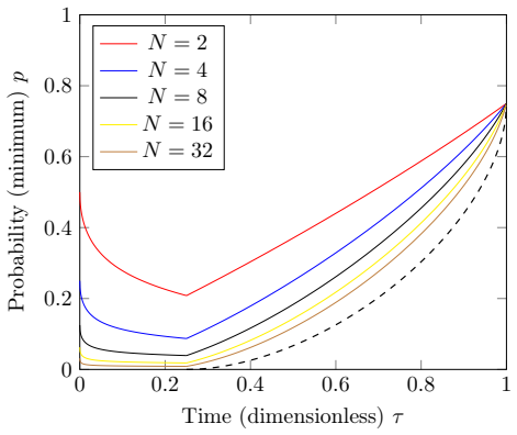
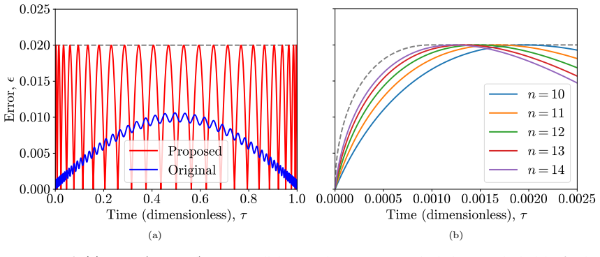
The central claim is that the schedule $s(\tau)=\frac12\left(1+\frac{2\tau-1}{\sqrt{1+4(N-1)\tau(1-\tau)}}\right)$ (Eq. 33) is a valid, near-optimal adiabatic schedule for unstructured search. It is obtained by saturating the adiabatic condition with the exact transition matrix element $|\langle\varepsilon_1(s)|H'(s)|\varepsilon_0(s)\rangle|={\sqrt{N-1}}/({N g(s)})$ rather than the constant upper bound used by Roland and Cerf. The full evolution time becomes $T=2\sqrt{N-1}/\varepsilon=O(\sqrt{N})$, matching Grover and the original schedule. In the ideal errorless limit the marked-state probability obeys $q(\tau)=\frac{1}{2N}\left(1+2(N-1)\tau+\sqrt{1+4(N-1)\tau(1-\tau)}\right)$, which inverts to $\tau\le q$, so probability grows at least proportionally to time from arbitrarily small times. This linear growth is what permits the time--space tradeoff in the ideal case and motivates Protocol 1. Numerically, the exact error for the two-level reduced Schrödinger system stays below $\varepsilon$, and the measured probability beats the original schedule until roughly halfway and beats Grover after a constant physical time.
Load-bearing premise
The paper assumes the pointwise adiabatic theorem, Theorem 1, holds for this specific Hamiltonian: satisfying the adiabatic condition of Eq. (13) with parameter $\varepsilon$ guarantees ground-state probability at least $1-\varepsilon^2$ at every dimensionless time, and because the schedule is built by saturating exactly that condition, the adiabaticity of Eq. (33) and the guarantee of Protocol 1 collapse if that implication fails.
Editorial extensions
If this is right
- Full evolution under Eq. (33) takes $T=2\sqrt{N-1}/\varepsilon$, preserving the $O(\sqrt{N})$ quadratic speedup of Grover's algorithm.
- In the errorless ideal limit, marked-state probability satisfies $\tau\le q$, so a measurement at any early time has a chance that grows linearly with time; for the original schedule and Grover the early probability is only $\cos^2((1-\tau)\arccos(1/\sqrt{N}))$.
- Protocol 1 guarantees a marked-state probability of at least $p$ in time $O(\sqrt{N}(1+p/\varepsilon))$, with constant-time trivial output when $p\le 1/N$.
- Numerical evidence for $n$ up to 40 shows adiabaticity with error bounded by $\varepsilon$, and the new schedule outscores the original schedule before halfway and Grover after a constant crossover time $t_{\mathrm{cross}}=O(1)$.
- With bounded coherence time, Grover's algorithm and the original schedule lose quantum advantage, while the new schedule can retain $O(\sqrt{N})$ running time provided coherence exceeds a constant.
Reading between the lines
- Beyond the paper: the derivation tactic of saturating the adiabatic condition with the exact matrix element, rather than a worst-case bound, should transfer to other two-level adiabatic search problems whose gap and transition element are known; the paper only carries it out for the symmetric $\{|m\rangle, |m^\perp\rangle\}$ subspace.
- Beyond the paper: the ideal linear relation $\tau\le q$ shows that a hypothetical schedule with error $\epsilon(\tau)\propto\sqrt{\tau}$ would make Theorem 3's perfect time--space tradeoff physically real; the numerical errors here asymptotically exceed that bound, but the general possibility remains open for other schedules.
- Beyond the paper: the constant crossover time $t_{\mathrm{cross}}=O(1)$ against Grover suggests that the practical resource for early-termination cryptographic races is the constant per-iteration overhead $k$ in Eq. (71), not the database size $N$.
- Beyond the paper: Protocol 1's minimum coherence time currently scales as $O(\sqrt{N})$; a tighter finite-$N$ bound exploiting the sine-square-root error function could plausibly remove this, which the authors themselves flag as future work.
Editorial analysis
A structured set of objections, weighed in public.
Referee Report
Summary. The paper proposes a new adiabatic schedule s(τ) for unstructured search, Eq. (33), derived by saturating the pointwise adiabatic condition with the exact transition matrix element. It claims O(√N) full evolution, a marked-state probability that in the ideal errorless limit grows as q≈τ (Eq. (40)), superior early-time probability relative to Roland–Cerf and Grover, and a Protocol 1 guaranteeing probability at least p in time 2√(N−1)(1+p/ε)+O(1). The authors derive an exact 2D reduction of the Schrödinger equation (Appendix E) and simulate it up to n=40, observing errors bounded by ε and apparently also by the conjectured sine–square-root function Eq. (52). They analyze bounded-coherence and limited-parallelism scenarios, and conclude that constant-time perfect parallelization remains impossible under their conjectured error function, while early termination may still be useful.
Significance. If the schedule and the assumed adiabaticity hold, the paper identifies a genuinely new schedule with clean analytical ideal-limit behavior, parameter-free derivations, and a practical early-termination protocol. The algebraic derivation of the schedule and of q(τ), the exact 2D invariant-subspace reduction in Appendix E, and the numerical study up to n=40 are concrete strengths. The two load-bearing theoretical steps are not proven, however: the pointwise adiabatic theorem (Theorem 1) used in Protocol 1, and the conjectured sine–square-root error bound Eq. (52) used to argue against ideal parallelization. The authors acknowledge both limitations, but they are central to the paper's formal guarantees. The paper is therefore best read as a candidate schedule with strong numerical support and conditional protocols, rather than as a fully proven algorithmic claim.
major comments (3)
- [§2.3 and Protocol 1 (Eqs. (13)–(14), (67))] The guarantee of Protocol 1 is not rigorously established. Despite being labelled a theorem, Theorem 1 is immediately qualified by the Remark that sufficient conditions are unknown and that counterexamples exist [6–9]. Since the schedule Eq. (33) is obtained by saturating Eq. (13) pointwise, the construction lives exactly in the regime where the pointwise adiabatic condition is known to be insufficient. The numerical evidence in Figs. 9–10 covers finite N and fixed ε, so it cannot prove the all-N, 0<ε≪1 statement asserted by the protocol. Please either prove a rigorous adiabatic estimate for this specific Hamiltonian (for example under the assumptions of Jansen–Ruskai–Seiler) or explicitly reformulate Theorem 1 and Protocol 1 as conditional/conjectural throughout the paper, adjusting the abstract and protocol statement accordingly.
- [§4.2.3, §5, §7 (Eq. (52))] The paper's negative conclusion that perfect parallelization is not physically realizable depends on the conjectured sine–square-root error bound Eq. (52). Figure 9b shows numerical convergence from below for n≤14, and §7 explicitly states that this evidence is not a mathematical proof. Because this conjecture is used to conclude that the ideal linear q(τ) behavior cannot be realized in practice, that conclusion should be presented as a conjecture rather than as a formal result. To settle the parallelization question, a rigorous error bound (or a proof that no such bound exists) would be needed.
- [§6 and Eq. (76)] The bounded-coherence advantage described in the introduction and in Section 6 is not demonstrated. Protocol 1 requires t_f = 2√(N−1)(1+p/ε), so the only proven protocol needs coherence time Θ(√N) whenever p>1/N; the case of constant (N-independent) coherence time is explicitly deferred to Future work in Section 7. The O(√N) running time in Eq. (79) therefore does not establish an advantage over Grover's algorithm in the constant-coherence regime—it describes a different parameter regime. Please clearly separate the proven O(√N)-time protocol from the speculative constant-time regime.
minor comments (4)
- [§2.4, text below Eq. (16)] The sentence 'The ground states of H0 and H1 are |m⟩ and |ϕ⟩ respectively' has the two states reversed: H0=I−|ϕ⟩⟨ϕ| has ground state |ϕ⟩, while H1=I−|m⟩⟨m| has ground state |m⟩. This typo in a central section is easy to fix but could confuse readers.
- [§5.1, Eq. (70) and surrounding text] The derivation of Eq. (70) from the equality T_g = k T_a should be written out. As displayed, the expression with arccsc(√N_g) and the claimed approximation ε ≈ (8k/π)√(N_a/N_g) do not transparently match, and the '-2' term is not clearly part of the denominator or a separate subtraction.
- [Abstract and §4.1] The phrase 'increases directly proportional to time' should be qualified: Eq. (40) gives q≈τ in dimensionless time, so the physical-time proportionality constant is T=O(√N), not N-independent. This distinction matters for the subsequent parallelization discussion.
- [Figure 9 caption] The caption states that the numerics 'confirm adiabaticity as predicted by Theorem 1'; given the caveats in the Remark of §2.3, it would be more precise to say that the data are consistent with the assumed pointwise bound for the tested parameters.
Circularity Check
No circularity found: the schedule is derived from the adiabatic condition and the ideal linear probability is an algebraic consequence, not an input; the central guarantee is conditional on an acknowledged unproved theorem, which is a rigor concern rather than circularity.
full rationale
The derivation chain is algebraic and self-contained. The proposed schedule Eq. (33) is obtained by saturating the pointwise adiabatic condition Eq. (13) with the exact transition matrix element Eq. (24), and the ideal-probability relation Eq. (40), whose large-N limit gives q approximately tau, is a direct algebraic consequence of substituting that schedule into Eq. (34); it is not imposed as an input. Protocol 1 then uses the loose bound Eq. (48), derived in Appendix D from the constant-error case of Eq. (47), to convert the assumed adiabatic error bound into a time-to-probability guarantee. No parameter is fitted to data and then renamed a prediction; the conjectured sine-square-root error function of Section 4.2.3 is explicitly labeled a conjecture and is used only to argue that ideal parallelization is not physically realized. The only self-citation appears in related work on NISQ-inspired algorithms and is not load-bearing. The paper itself flags the main caveat: the Remark after Theorem 1 states that sufficient conditions for the pointwise adiabatic theorem are unknown and cites counterexamples, and Section 7 states that the numerical evidence does not constitute a mathematical proof. These are conditionality and rigor concerns, not circularity: the guarantee in Protocol 1 is conditional on Theorem 1 and on the numerical support, rather than being equivalent to its own inputs by construction. No circular step is therefore identified.
Assumptions & free parameters
assumptions (3)
- domain assumption The pointwise adiabatic theorem (Theorem 1) holds for the unstructured search Hamiltonian.
- domain assumption Initial state preparation and final measurement take constant time and are error-free.
- ad hoc to paper The conjectured sine-square-root error bound (Eq. 52) holds for the exact evolution.
Cite this review
Pith. "Pith review of Adiabatic quantum unstructured search in parallel." pith.science (2026). https://pith.science/paper/DT4RTIFD
@misc{pith2026250208594,
  author       = {Pith},
  title        = {Pith review of: Adiabatic quantum unstructured search in parallel},
  year         = {2026},
  howpublished = {\url{https://pith.science/paper/DT4RTIFD}},
  note         = {Machine review of arXiv:2502.08594}
}
abstract
We present an optimized adiabatic quantum schedule for unstructured search building on the original approach of Roland and Cerf [Phys. Rev. A 65, 042308 (2002)]. Our schedule adiabatically varies the Hamiltonian even more rapidly at the endpoints of its evolution, preserving Grover's well-known quadratic quantum speedup. In the errorless adiabatic limit, the probability of successfully obtaining the marked state from a measurement increases directly proportional to time, suggesting efficient parallelization. Numerical simulations of an appropriate reduced two-dimensional Schr\"odinger system confirm adiabaticity while demonstrating superior performance in terms of probability compared to existing adiabatic algorithms and Grover's algorithm, benefiting applications with possible premature termination. We introduce a protocol that ensures a marked-state probability at least $p$ in time of order $\sqrt{N}(1+p/\varepsilon)$, and analyze its implications for realistic bounded-resource scenarios. Our findings suggest that quantum advantage may still be achievable under constrained coherence times (where other algorithms fail), provided the hardware allows for them to be sufficiently long.
Figures


Figures from the paper (8 more)






Reference graph
Works this paper leans on
-
[1]
A fast quantum mechanical algorithm for database search
L. K. Grover, “A fast quantum mechanical algorithm for database search”, in Proceedings of the twenty-eighth annual ACM symposium on theory of computing, STOC ’96 (July 1996), pp. 212–219
1996
-
[2]
Strengths and weaknesses of quantum computing
C. H. Bennett, E. Bernstein, G. Brassard, and U. Vazirani, “Strengths and weaknesses of quantum computing”, SIAM J. Comput.26, 1510–1523 (1997)
1997
- [3]
-
[4]
M. Born and V. Fock, “Beweis des adiabatensatzes”, Zeitschrift für Physik51, 165–180 (1928)
work page 1928
-
[5]
Quantum search by local adiabatic evolution
J. Roland and N. J. Cerf, “Quantum search by local adiabatic evolution”, Phys. Rev. A65, 042308 (2002)
2002
-
[6]
Inconsistency in the application of the adiabatic theorem
K.-P. Marzlin and B. C. Sanders, “Inconsistency in the application of the adiabatic theorem”, Phys. Rev. Lett.93, 160408 (2004)
work page 2004
-
[7]
Quantitative conditions do not guarantee the validity of the adiabatic approximation
D. Tong, K. Singh, L. C. Kwek, and C. H. Oh, “Quantitative conditions do not guarantee the validity of the adiabatic approximation”, Phys. Rev. Lett.95, 110407 (2005)
work page 2005
-
[8]
Experimental study of the validity of quantitative conditions in the quantum adiabatic theorem
J. Du, L. Hu, Y. Wang, J. Wu, M. Zhao, and D. Suter, “Experimental study of the validity of quantitative conditions in the quantum adiabatic theorem”, Phys. Rev. Lett.101, 060403 (2008)
work page 2008
Show all 27 references
-
[9]
Adiabatic condition and quantum geometric poten- tial
J. Wu, M. Zhao, J. Chen, and Y. Zhang, “Adiabatic condition and quantum geometric poten- tial”, Phys. Rev. A77, 062114 (2008)
2008
-
[10]
Analog analogue of a digital quantum computation
E. Farhi and S. Gutmann, “Analog analogue of a digital quantum computation”, Phys. Rev. A 57, 2403–2406 (1998)
1998
-
[11]
Grover’s quantum searching algorithm is optimal
C. Zalka, “Grover’s quantum searching algorithm is optimal”, Phys. Rev. A60, 2746–2751 (1999)
1999
-
[12]
On the adiabatic theorem of quantum mechanics
T. Kato, “On the adiabatic theorem of quantum mechanics”, J. Phys. Soc. Jpn.5, 435–439 (1950)
1950
-
[13]
Bounds for the adiabatic approximation with appli- cations to quantum computation
S. Jansen, M.-B. Ruskai, and R. Seiler, “Bounds for the adiabatic approximation with appli- cations to quantum computation”, J. Math. Phys.48, 10.1063/1.2798382 (2007)
2007 doi
-
[14]
A note on the switching adiabatic theorem
A. Elgart and G. A. Hagedorn, “A note on the switching adiabatic theorem”, J. Math. Phys. 53, 10.1063/1.4748968 (2012)
2012 doi
-
[15]
Rapidadiabaticpreparationofinjectiveprojectedentangled pair states and Gibbs states
Y.Ge,A.Molnár,andJ.I.Cirac,“Rapidadiabaticpreparationofinjectiveprojectedentangled pair states and Gibbs states”, Phys. Rev. Lett.116, 080503 (2016)
2016
-
[16]
Garcia-Saez and J
A. Garcia-Saez and J. I. Latorre,Addressing hard classical problems with adiabatically assisted variational quantum eigensolvers, June 2018, arXiv:1806.02287 [quant-ph]
2018 arXiv
-
[17]
Improving the variational quantum eigensolver using variational adiabatic quantum computing
S. M. Harwood, D. Trenev, S. T. Stober, P. Barkoutsos, T. P. Gujarati, S. Mostame, and D. Greenberg, “Improving the variational quantum eigensolver using variational adiabatic quantum computing”, ACM Transactions on Quantum Computing3, 1–20 (2022). 25
2022
-
[18]
Simulatingadiabaticquantumcom- puting with parameterized quantum circuits
I.Kolotouros,I.Petrongonas,M.Prokop,andP.Wallden,“Simulatingadiabaticquantumcom- puting with parameterized quantum circuits”, Quantum Science and Technology10, 015003 (2024)
2024
-
[19]
Adiabatic quantum computation
T. Albash and D. A. Lidar, “Adiabatic quantum computation”, Rev. Mod. Phys.90, 015002 (2018)
2018
-
[20]
Beitragzurnäherungsweisenintegrationtotalerdifferentialgleichungen
W.Kutta,“Beitragzurnäherungsweisenintegrationtotalerdifferentialgleichungen”,Zeitschrift für Mathematik und Physik46, 435–453 (1901)
1901
-
[21]
A family of embedded Runge–Kutta formulae
J. R. Dormand and P. J. Prince, “A family of embedded Runge–Kutta formulae”, J. Comput. Appl. Math.6, 19–26 (1980)
1980
-
[22]
Some practical Runge–Kutta formulas
L. F. Shampine, “Some practical Runge–Kutta formulas”, Math. Comput.46, 135–150 (1986)
1986
-
[23]
SciPy 1.0: Fundamental Algorithms for Scientific Computing in Python
P. Virtanen, R. Gommers, T. E. Oliphant, M. Haberland, T. Reddy, D. Cournapeau, E. Burovski, P. Peterson, W. Weckesser, J. Bright, S. J. van der Walt, M. Brett, J. Wilson, K. J. Millman, N. Mayorov, A. R. J. Nelson, E. Jones, R. Kern, E. Larson, C. J. Carey, İ. Polat, Y. Feng,...
2020
-
[24]
Tightboundsonquantumsearching
M.Boyer,G.Brassard,P.Høyer,andA.Tapp,“Tightboundsonquantumsearching”,Fortschritte der Physik: Progress of Physics46, 493–505 (1998)
1998
-
[25]
On the exponential solution of differential equations for a linear operator
W. Magnus, “On the exponential solution of differential equations for a linear operator”, Com- mun. Pure Appl. Math.7, 649–673 (1954)
1954
-
[26]
Quantum search with hybrid adiabatic– quantum-walk algorithms and realistic noise
J. G. Morley, N. Chancellor, S. Bose, and V. Kendon, “Quantum search with hybrid adiabatic– quantum-walk algorithms and realistic noise”, Phys. Rev. A99, 022339 (2019)
2019
-
[27]
Accuracy versus run time in an adiabatic quantum search
A. T. Rezakhani, A. K. Pimachev, and D. A. Lidar, “Accuracy versus run time in an adiabatic quantum search”, Phys. Rev. A82, 052305 (2010). 26
2010
Reviewed August 8, 2026 · model on record in the stance chip above.
Discussion (0). Continue with ORCID to comment.