REVIEW 3 major objections 5 minor 49 references
A Three-Feature Model to Predict Colour Change Blindness
T0 review · 3 major / 5 minor · reviewed 2026-08-14 · deepseek-v4-flash
Pith's one-line read Three features predict how long a colour change goes unnoticed.
desk verdict Useful benchmark and honest simple model, but the headline correlations rest on a post hoc mode target and an empirically chosen threshold. read the letter →
The pith
A machine-rendered reading of the paper's core claim, the machinery that carries it, and where it could break.
The reading
What carries the argument
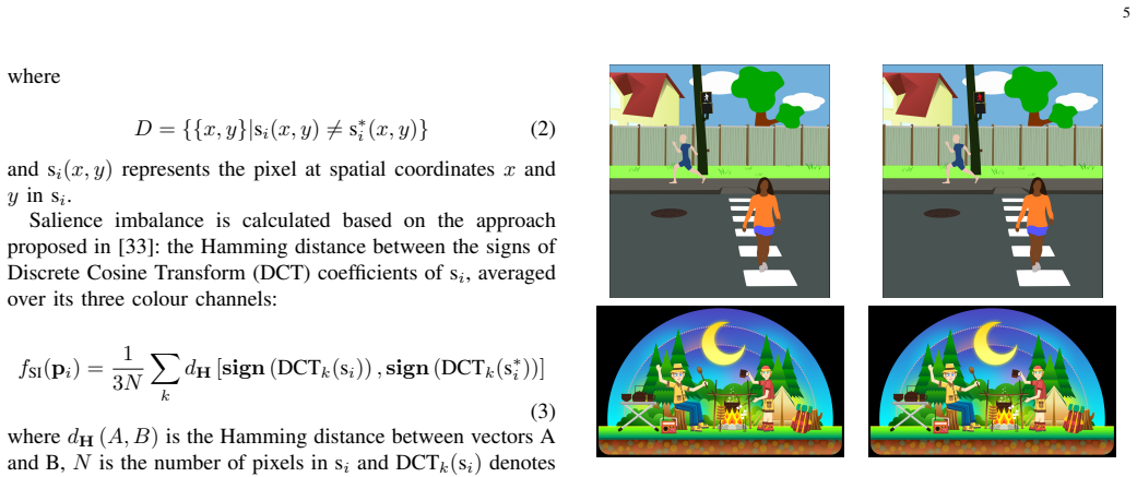
The carrying object is the three-term linear regressor $\tilde{T}_i = b_1 f_{CM} + b_2 f_{SI} + b_3 f_{UE}$, with only the three coefficients fitted. $f_{CM}$ is the mean LAB2000HL Euclidean colour distance over the changed pixels only; $f_{SI}$ is the average, across the three colour channels, of the Hamming distance between the signs of DCT coefficients of the original and changed images, a measure of salience imbalance; $f_{UE}$ is the squared average over observers of the pair's rank in each observer's random trial sequence, representing short-term learning. The regression target is the dominant mode $\hat{T}_i$ of each pair's detection times, chosen because the modes split into two clusters at 36 seconds. The same feature triple, fed to quadratic discriminant analysis, is what yields the 85% easy/hard classification.
What would settle it
Collect detection times for a fresh, independent set of cartoon pairs using the same flicker protocol and check whether per-pair distributions still have a single dominant mode and whether those modes still form two clusters separated near 36 seconds. If the bimodal structure does not reappear, the regression target and the 85% classification accuracy are tied to this dataset; a cheaper check is to refit the three features against mean detection times and see whether the correlation advantage over individual features survives.
Extended reading notes
Core claim
The central claim is that the difficulty of noticing a single colour change is not best summarised by the mean detection time, but by the dominant mode of the detection-time distribution, and that this mode is predictable from two image-computable features plus experience. After collecting 3418 valid detection times, the paper finds every pair's distribution is non-normal with one dominant peak, and the modes form two natural clusters separated by a density minimum at about 36 seconds. Regression on change magnitude, salience imbalance, and experience reaches PLCC 0.62 and SROCC 0.63 against mode detection times, significantly better than each feature alone and than the existing model [31], which scores 0.39. The same three features, used in quadratic discriminant analysis, classify pairs into the two mode-based clusters with 85% accuracy; a four-node decision tree achieves 78% and reveals that the hardest pairs combine low experience with large colour changes, or high experience with a large change and weak salience imbalance.
Load-bearing premise
The load-bearing premise is that the dominant mode of each pair's detection times, a statistic selected after seeing the data, is the correct measure of that pair's difficulty, and that the 36-second gap between two mode clusters is a stable property of change blindness rather than a product of this particular dataset and threshold choice.
Editorial extensions
If this is right
- A fully automatic pipeline can rank any collection of single-colour-change image pairs from easiest to hardest without eye tracking, manual annotation, or per-image parameter tuning.
- Because the experience feature is simply trial count, adaptive experiments or games could schedule stimulus difficulty around the observer's accumulated practice.
- Linear pooling of the three features is not significantly worse than support vector regression, a neural network, or a decision tree, so the operational model stays at three fitted parameters.
- The released benchmark includes the per-observer stimulus order, enabling other groups to model experience and practice effects that earlier public change-blindness data lacked.
Reading between the lines
- If the salience-imbalance feature works because sign flips of DCT coefficients flag local spectral change, a learned salience difference on natural photographs might substitute for it, extending the same three-term model beyond cartoons.
- The two mode clusters hint at two observer subpopulations — one fast and one slow — so modelling the clusters separately, rather than pooling everyone, could raise the ceiling above the reported correlations.
- Because the experience feature enters as a squared average rank, the model suggests that detection-time noise grows for pairs shown out of order relative to the group average, which an experiment designer could exploit by randomising more aggressively when estimating modes.
Signed reviews
Editorial analysis
A structured set of objections, weighed in public.
Referee Report
Summary. The paper introduces a three-feature linear regression model for predicting colour change blindness in cartoon image pairs viewed under a flicker paradigm. The features are change magnitude (mean perceived colour difference over the changed pixels), salience imbalance (Hamming distance between DCT sign patterns of the two images, averaged over colour channels), and user experience (squared average of the stimulus rank in each observer's random sequence). The target statistic is the dominant mode of the per-pair detection-time distribution, selected after observing that detection times are non-normal and often multimodal. On a dataset of 100 image pairs and 60 valid observers, the model is reported to predict mode detection times with PLCC 0.62 and SROCC 0.63 under 100 random 70/30 splits, outperforming individual features, the Ma et al. model, and other regressors. The paper also reports binary classification of stimuli into easy/hard classes with 85% accuracy using quadratic discriminant analysis with ten-fold cross-validation, where the difficulty threshold is placed at the density minimum of the mode distribution.
Significance. The paper makes two concrete contributions: a new publicly available change-blindness benchmark with controlled collection conditions and observer ranks, and a simple, fully automatic predictive model with only three parameters. The strengths are the clean experimental setup, the explicit cross-validation protocol with 100 random splits, the fair comparison with several baselines, and the placement of the dataset in the public domain. If the mode-based target and the threshold-based difficulty classes were justified a priori, the model would be a practically useful tool for ranking and classifying the difficulty of spot-the-difference stimuli. However, the central quantitative claims (correlations of approximately 0.62 and classification accuracy of 85%) are obtained for a target statistic and a threshold that were chosen after inspecting the same data used for evaluation, and the mode estimate itself is noisy given only 21-41 observations per pair. This post hoc selection is the main threat to the validity of the reported performance and should be addressed before the results can be taken at face value.
major comments (3)
- [III-A2] The choice of the dominant mode as the regression target is made post hoc. Section III-A2 states that the mean detection time does not produce clearly separated clusters, and therefore the dominant mode is selected as the target. This means the fitted regression target in Eq. (5) is itself a statistic chosen from the observed data. With only 21-41 observations per image pair, the sample mode is unstable, and a target selected to produce clean clusters can inflate the reported correlations (Table II, PLCC 0.62 / SROCC 0.63). Please provide an a priori definition of the target statistic, or validate the mode-based analysis on an independent hold-out set with the target fixed before any model fitting.
- [III-A2 / IV-B] The classification threshold is inconsistent and data-derived. Section III-A2 defines Tcrit = 36 s as the global density minimum of the mode distribution, but Section IV-B reports classification using a 35 s threshold, and Figure 3's caption mentions 'around 35s'. Moreover, the threshold is derived from the same data used to evaluate the 85% classification accuracy. Because the classes C1 and C2 are defined by this threshold, the accuracy partly reflects a fit to the data. Please report classification results with a pre-specified threshold (e.g., 36 s fixed before analysis, or a threshold chosen on the training folds only, with the test folds evaluated using that threshold) and clarify the discrepancy between 35 s and 36 s.
- [Table II] The paper's practical claim rests on the mode-based target, yet the model's correlation with individual detection times is only PLCC 0.29 and SROCC 0.29. The abstract and introduction frame the model as 'predict[ing] colour change blindness' and 'predict[ing] detection times', which a reader would naturally interpret as individual-trial detection times. The gap between individual-level and mode-level performance should be discussed explicitly, and the claims should be qualified as applying to a summary statistic of each pair rather than to individual observers.
minor comments (5)
- [III-A2] The Kolmogorov-Smirnov test is described as being applied 'at the 5% confidence level'; the correct terminology is 'significance level'.
- [Eq. (1)] The notation `#D` in Eq. (1) is used without a prior definition; please define it as the number of changed pixels.
- [Figure 3] The caption of Figure 3 says 'around 35s', while the text in Section III-A2 gives 36 s; please make the numbers consistent.
- [Section IV-A] The sentence 'we trained the three parameters of Eqn. (2) in [31]' is unclear because Eq. (2) in the cited paper [31] is not reproduced here; please briefly describe the Ma et al. model or its parametrisation.
- [Section III-B] The definition of fUE in Eq. (4) as the squared average rank deserves a one-sentence justification; as written, the squaring seems arbitrary and is not motivated in the text.
Circularity Check
Regression is self-contained; the 85% classification result is partially circular because the difficulty labels and threshold are derived from the same mode detection times used as ground truth.
-
self definitional
[Section III-A2 (target and class definition) and Section IV-B (classification evaluation)]
"The two naturally emerging clusters C1 and C2 were then used as ground truth for our classification analysis: C1 = {pi|i : ˆTi < Tcrit} ... where Tcrit is the critical time (minimum density of DT modes): 36 s. ... Image pairs were classified depending on whether ˆT (i) was below or above 35 seconds ( C1 or C2). ... A ten-fold cross-validation gave an average overall accuracy of 85% to classify mode detection times."
The classification ground truth is not an independent, pre-specified criterion: C1 and C2 are defined by thresholding the measured mode detection times T_hat_i at the density minimum of those same T_hat_i values. The 85% accuracy is then evaluated against these data-derived labels. The threshold is also inconsistent (36 s in the definition, 35 s in the evaluation), indicating that the label boundary is fitted to the data rather than fixed a priori. Consequently, the classification claim partly reports how well the features recover a threshold chosen from the very data being predicted, rather than predicting an externally defined difficulty class. The regression correlations are not affected because fCM, fSI, and fUE are computed independently of the detection-time values.
full rationale
The core regression model is self-contained: the features (change magnitude from LAB2000HL, salience imbalance from DCT sign Hamming distance, and user experience from sequence rank) are all computed from the images and experimental design, not from the detection times, and the PLCC/SROCC values are obtained by 70/30 cross-validation. No load-bearing step is justified only by a self-citation: the citation of Hou et al. is external, and the authors' own prior work appears only as context or as an alternative feature source. The only genuine circularity concern is the classification evaluation, where the difficulty labels are defined from the same mode detection times that serve as the prediction target. That makes the 85% accuracy a partially in-sample assessment of a data-driven label definition. This warrants a moderate score of 4; the central regression claim retains independent content.
Assumptions & free parameters
free parameters (4)
- b1 (regression coefficient for change magnitude) =
not reported
- b2 (regression coefficient for salience imbalance) =
not reported
- b3 (regression coefficient for user experience) =
not reported
- Tcrit (classification threshold) =
36 s
assumptions (4)
- domain assumption Cartoon images provide robust scene and object attributes that are not reliant on noisy low-level feature extractors.
- domain assumption LAB2000HL is a perceptually uniform and hue-linear colour space, so Euclidean distance in it approximates just noticeable difference.
- ad hoc to paper The dominant mode of detection times is a more appropriate target statistic than the mean for representing change blindness.
- domain assumption The flicker paradigm (800ms display, 80ms flicker) induces change blindness as described.
Cite this review
Pith. "Pith review of A Three-Feature Model to Predict Colour Change Blindness." pith.science (2026). https://pith.science/paper/EKQN73IX
@misc{pith2026190904147,
  author       = {Pith},
  title        = {Pith review of: A Three-Feature Model to Predict Colour Change Blindness},
  year         = {2026},
  howpublished = {\url{https://pith.science/paper/EKQN73IX}},
  note         = {Machine review of arXiv:1909.04147}
}
read the original abstract
Change blindness is a striking shortcoming of our visual system which is exploited in the popular "Spot the difference" game. It makes us unable to notice large visual changes happening right before our eyes and illustrates the fact that we see much less than we think we do. We introduce a fully automated model to predict colour change blindness in cartoon images based on two low-level image features and observer experience. Using linear regression with only three parameters, the predictions of the proposed model correlate significantly with measured detection times. We also demonstrate the efficacy of the model to classify stimuli in terms of difficulty.
Figures


Figures from the paper (2 more)

Reference graph
Works this paper leans on
-
[1]
Daniel J Simons and Daniel T Levin, “Change blindness,” Trends in cognitive sciences, vol. 1, no. 7, pp. 261–267, 1997
work page 1997
-
[2]
Change blindness and inattentional blindness,
M.S. Jensen, R. Yao, W.N. Street, and D.J. Simons, “Change blindness and inattentional blindness,” Wiley Interdiscip. Rev. Cognit. Sci., vol. 2, no. 5, pp. 529–546, 2011
work page 2011
-
[3]
What is the bandwidth of perceptual experience?,
M. A. Cohen, D. C. Dennett, and N. Kanwisher, “What is the bandwidth of perceptual experience?,” Trends in Cognitive Sciences , vol. 20, no. 5, pp. 324–335, 2016
work page 2016
-
[4]
Exploring the informational sources of metaperception: The case of change blindness blindness,
Anna Loussouarn, Damien Gabriel, and Jo ¨elle Proust, “Exploring the informational sources of metaperception: The case of change blindness blindness,” Consciousness and cognition, vol. 20, no. 4, pp. 1489–1501, 2011
work page 2011
-
[5]
Change blindness in driving scenes,
Adam Galpin, Geoffrey Underwood, and David Crundall, “Change blindness in driving scenes,” Transportation research part F: traffic psychology and behaviour , vol. 12, no. 2, pp. 179–185, 2009
work page 2009
-
[6]
Cell phone conversing while driving in new zealand: Prevalence, risk perception and legislation,
Charlene Hallett, Anthony Lambert, and Michael A Regan, “Cell phone conversing while driving in new zealand: Prevalence, risk perception and legislation,” Accident Analysis & Prevention , vol. 43, no. 3, pp. 862–869, 2011
work page 2011
-
[7]
Identifying macrocognitive function failures from accident reports: a case study,
Peng Liu, Xi Lyu, Yongping Qiu, Juntao Hu, Jiejuan Tong, and Zhizhong Li, “Identifying macrocognitive function failures from accident reports: a case study,” in Advances in Human Factors in Energy: Oil, Gas, Nuclear and Electric Power Industries , pp. 29–40. Springer, 2017
work page 2017
-
[8]
Military in curb on civilian visits,
E. Sciolino, “Military in curb on civilian visits,” New York Times, 2001
work page 2001
Show all 49 references
-
[9]
Change blindness and eyewitness testimony,
Graham Davies and Sarah Hine, “Change blindness and eyewitness testimony,” The Journal of psychology , vol. 141, no. 4, pp. 423–434, 2007
2007
-
[10]
Varying rendering fidelity by exploiting human change blindness,
Kirsten Cater, Alan Chalmers, and Colin Dalton, “Varying rendering fidelity by exploiting human change blindness,” in Proceedings of the 1st international conference on Computer graphics and interactive techniques in Australasia and South East Asia , Melbourne, Australia, Febru...
2003
-
[11]
Leveraging change blindness for redirection in virtual environments,
Evan A Suma, Seth Clark, David Krum, Samantha Finkelstein, Mark Bolas, and Zachary Warte, “Leveraging change blindness for redirection in virtual environments,” in Virtual Reality Conference (VR), 2011 IEEE. IEEE, 2011, pp. 159–166
2011
-
[12]
Towards exploiting change blindness for image processing,
Steven Le Moan, Ivar Farup, and Jana Blahov ´a, “Towards exploiting change blindness for image processing,” Journal of Visual Communica- tion and Image Representation , vol. 54, pp. 31–38, 2018
2018
-
[13]
Autopager: exploiting change blindness for gaze-assisted reading,
Andrew D Wilson and Shane Williams, “Autopager: exploiting change blindness for gaze-assisted reading,” in Proceedings of the 2018 ACM Symposium on Eye Tracking Research & Applications . ACM, 2018, p. 46
2018
-
[14]
Change blindness in proximity-aware mobile interfaces,
Michael Brock, Aaron Quigley, and Per Ola Kristensson, “Change blindness in proximity-aware mobile interfaces,” in Proceedings of the 2018 CHI Conference on Human Factors in Computing Systems . ACM, 2018, p. 43
2018
-
[15]
Adopting abstract images for semantic scene understanding,
C.L. Zitnick, R. Vedantam, and D. Parikh, “Adopting abstract images for semantic scene understanding,” IEEE Trans. Pattern Anal. Mach. Intell., vol. 38, no. 4, pp. 627–638, 2016
2016
-
[16]
The principles of psychology, vol. 2. ny, us: Henry holt and company,
W James, “The principles of psychology, vol. 2. ny, us: Henry holt and company,” 1890
-
[17]
Local masking in natural images: A database and analysis,
Md Mushfiqul Alam, Kedarnath P Vilankar, David J Field, and Da- mon M Chandler, “Local masking in natural images: A database and analysis,” Journal of vision , vol. 14, no. 8, pp. 22–22, 2014
2014
-
[18]
A psychophysical evaluation of texture compression masking effects,
Guillaume Lavou ´e, Michael Langer, Adrien Peytavie, and Pierre Poulin, “A psychophysical evaluation of texture compression masking effects,” IEEE transactions on visualization and computer graphics , vol. 25, no. 2, pp. 1336–1346, 2018
2018
-
[19]
Global transsaccadic change blindness during scene perception,
John M Henderson and Andrew Hollingworth, “Global transsaccadic change blindness during scene perception,” Psychological science, vol. 14, no. 5, pp. 493–497, 2003
2003
-
[20]
Change- blindness as a result of ‘mudsplashes’,
J Kevin O’Regan, Ronald A Rensink, and James J Clark, “Change- blindness as a result of ‘mudsplashes’,” Nature, vol. 398, no. 6722, pp. 34–34, 1999
1999
-
[21]
As if by magic: An abrupt change in motion direction induces change blindness,
Richard Yao, Katherine Wood, and Daniel J Simons, “As if by magic: An abrupt change in motion direction induces change blindness,” Psychological science, vol. 30, no. 3, pp. 436–443, 2019
2019
-
[22]
Change blindness in the absence of a visual disruption,
Daniel J Simons, Steven L Franconeri, and Rebecca L Reimer, “Change blindness in the absence of a visual disruption,” Perception, vol. 29, no. 10, pp. 1143–1154, 2000
2000
-
[23]
Gorillas in our midst: Sustained inattentional blindness for dynamic events,
Daniel J Simons and Christopher F Chabris, “Gorillas in our midst: Sustained inattentional blindness for dynamic events,” perception, vol. 28, no. 9, pp. 1059–1074, 1999
1999
-
[24]
Posterior parietal cortex mediates encoding and maintenance processes in change blindness,
Philip Tseng, Tzu-Yu Hsu, Neil G Muggleton, Ovid JL Tzeng, Daisy L Hung, and Chi-Hung Juan, “Posterior parietal cortex mediates encoding and maintenance processes in change blindness,” Neuropsychologia, vol. 48, no. 4, pp. 1063–1070, 2010
2010
-
[25]
Information capacity of a single retinal channel,
D Kelly, “Information capacity of a single retinal channel,” IRE Transactions on Information Theory , vol. 8, no. 3, pp. 221–226, 1962
1962
-
[26]
How much the eye tells the brain,
Kristin Koch, Judith McLean, Ronen Segev, Michael A Freed, Michael J Berry II, Vijay Balasubramanian, and Peter Sterling, “How much the eye tells the brain,” Current Biology, vol. 16, no. 14, pp. 1428–1434, 2006
2006
-
[27]
Some studies in the speed of visual perception,
G Sziklai, “Some studies in the speed of visual perception,” IRE Transactions on Information Theory , vol. 2, no. 3, pp. 125–128, 1956
1956
-
[28]
Metamers of the ventral stream,
Jeremy Freeman and Eero P. Simoncelli, “Metamers of the ventral stream,” Nat. Neurosci., vol. 14, no. 9, pp. 1195–1201, 2011
2011
-
[29]
Neural correlates of change detection and change blindness in a working memory task,
Luiz Pessoa and Leslie G Ungerleider, “Neural correlates of change detection and change blindness in a working memory task,” Cerebral Cortex, vol. 14, no. 5, pp. 511–520, 2004
2004
-
[30]
Performance-optimized hierarchical models predict neural responses in higher visual cortex,
Daniel LK Yamins, Ha Hong, Charles F Cadieu, Ethan A Solomon, Dar- ren Seibert, and James J DiCarlo, “Performance-optimized hierarchical models predict neural responses in higher visual cortex,” Proceedings of the National Academy of Sciences , vol. 111, no. 23, pp. 8619–8624, 2014
2014
-
[31]
Change blindness images,
Li-Qian Ma, Kun Xu, Tien-Tsin Wong, Bi-Ye Jiang, and Shi-Min Hu, “Change blindness images,” Visualization and Computer Graphics, IEEE Trans. on , vol. 19, no. 11, pp. 1808–1819, 2013
2013
-
[32]
Spoid: a system to produce spot-the-difference puzzle images with difficulty,
Jung-Hwan Jin, Hyun Joon Shin, and Jung-Ju Choi, “Spoid: a system to produce spot-the-difference puzzle images with difficulty,” The Visual Computer, vol. 29, no. 6-8, pp. 481–489, 2013
2013
-
[33]
Image signature: Highlighting sparse salient regions,
Xiaodi Hou, Jonathan Harel, and Christof Koch, “Image signature: Highlighting sparse salient regions,” Pattern Analysis and Machine Intelligence, IEEE Trans. on , vol. 34, no. 1, pp. 194–201, 2012
2012
-
[34]
A semi-automated approach to balancing of bottom-up salience for predicting change detection performance,
Milan Verma and Peter W McOwan, “A semi-automated approach to balancing of bottom-up salience for predicting change detection performance,” Journal of vision , vol. 10, no. 6, pp. 3–3, 2010
2010
-
[35]
Is” change blindness
Steffen Werner and Bjorn Thies, “Is” change blindness” attenuated by domain-specific expertise? an expert-novices comparison of change detection in football images,” Visual Cognition , vol. 7, no. 1-3, pp. 163–173, 2000
2000
-
[36]
Change blindness, aging, and cognition,
Matthew Rizzo, JonDavid Sparks, Sean McEvoy, Sarah Viamonte, Ida Kellison, and Shaun P Vecera, “Change blindness, aging, and cognition,” Journal of clinical and experimental neuropsychology, vol. 31, no. 2, pp. 245–256, 2009. 8
2009
-
[37]
Culture and change blind- ness,
Takahiko Masuda and Richard E Nisbett, “Culture and change blind- ness,” Cognitive science, vol. 30, no. 2, pp. 381–399, 2006
2006
-
[38]
Individual differences in change blindness are predicted by the strength and stability of visual representations,
Nora Andermane, Jenny M Bosten, Anil K Seth, and Jamie Ward, “Individual differences in change blindness are predicted by the strength and stability of visual representations,” Neuroscience of consciousness , vol. 2019, no. 1, pp. niy010, 2019
2019
-
[39]
The capacity of visual short- term memory is set both by visual information load and by number of objects,
George A Alvarez and Patrick Cavanagh, “The capacity of visual short- term memory is set both by visual information load and by number of objects,” Psychological science, vol. 15, no. 2, pp. 106–111, 2004
2004
-
[40]
Change blindness is influenced by both contrast energy and subjective importance within local regions of the image,
Wietske Zuiderbaan, Jonathan van Leeuwen, and Serge O Dumoulin, “Change blindness is influenced by both contrast energy and subjective importance within local regions of the image,” Frontiers in psychology, vol. 8, pp. 1718, 2017
2017
-
[41]
VSI: A visual saliency induced index for perceptual image quality assessment,
L. Zhang, Y . Shen, and H. Li, “VSI: A visual saliency induced index for perceptual image quality assessment,” IEEE Trans. Image Process. , vol. 23, no. 10, pp. 4270–4281, 2014
2014
-
[42]
Cb database: A change blindness database for objects in natural indoor scenes,
Preeti Sareen, Krista A Ehinger, and Jeremy M Wolfe, “Cb database: A change blindness database for objects in natural indoor scenes,” Behavior research methods, vol. 48, no. 4, pp. 1343–1348, 2016
2016
-
[43]
thesis, Masarykova univerzita, Fakulta soci ´aln´ıch studi´ı, 2013
Michaela PORUBANOV ´A, Change Blindness and Its Determinants , Ph.D. thesis, Masarykova univerzita, Fakulta soci ´aln´ıch studi´ı, 2013
2013
-
[44]
Measuring visual clutter,
Ruth Rosenholtz, Yuanzhen Li, and Lisa Nakano, “Measuring visual clutter,” Journal of vision , vol. 7, no. 2, pp. 17–17, 2007
2007
-
[45]
Computational estimation of visual com- plexity,
ML Mack and A Oliva, “Computational estimation of visual com- plexity,” in The 12th annual object, perception, attention, and memory conference, 2004
2004
-
[46]
Predicting image differences based on image-difference features,
I. Lissner, J. Preiss, and P. Urban, “Predicting image differences based on image-difference features,” in IS&T/SID, 19th Color and Imaging Conference, San Jose, CA, 2011, pp. 23–28
2011
-
[47]
Toward a unified color space for perception-based image processing,
Ingmar Lissner and Philipp Urban, “Toward a unified color space for perception-based image processing,” IEEE Trans. on Image Processing, vol. 21, no. 3, pp. 1153–1168, 2012
2012
-
[48]
Can image quality features predict visual change blindness?,
Steven Le Moan, “Can image quality features predict visual change blindness?,” in 2017 International Conference on Image and Vision Computing New Zealand (IVCNZ) . IEEE, 2017, pp. 1–5
2017
-
[49]
Saccadic model of eye movements for free-viewing condition,
Olivier Le Meur and Zhi Liu, “Saccadic model of eye movements for free-viewing condition,” Vision research, vol. 116, pp. 152–164, 2015
2015
Reviewed August 14, 2026 · model on record in the stance chip above.
Discussion (0). Continue with ORCID to comment.