REVIEW 4 major objections 6 minor 41 references
Binary and Ternary Quantization Can Enhance Feature Discrimination
T0 review · 4 major / 6 minor · reviewed 2026-08-16 · deepseek-v4-flash
Pith's one-line read Coarse 1-bit and 2-bit quantization can sharpen class separation instead of degrading it, provided the threshold is chosen correctly.
desk verdict The scalar theory is solid and worth reviewing, but the paper's vector-level claim rests on an unproved aggregation step and overstates what the experiments show. read the letter →
The pith
A machine-rendered reading of the paper's core claim, the machinery that carries it, and where it could break.
The reading
What carries the argument
The load-bearing object is the discrimination ratio $D = E[(X_1-Y_1)^2] / ( E[(X_1-X_2)^2] + E[(Y_1-Y_2)^2] )$, a linear-discrimination quotient of inter-class to intra-class scatter, together with its quantized counterparts $D_b$ and $D_t$. Under the standardized Gaussian model of Property 1, the quantized moments collapse to polynomials in the standard-normal tail probabilities $\alpha = \Phi((\tau-\mu)/\sigma)$ and $\beta = \Phi((\tau+\mu)/\sigma)$, so the comparison $D_b > D$ or $D_t > D$ becomes a quadratic inequality in $\alpha$. Solving the quadratic and discarding the root that conflicts with $\alpha < \beta$ yields conditions (8) and (9), whose left-hand sides can be evaluated or minimized over $\tau$. This reduction is what turns a nonlinear quantizer into a solvable threshold-selection problem, and the same machinery supplies the gradient-descent recipe of Appendix B for locating enhancing thresholds.
What would settle it
Take a real feature set with strong inter-coordinate correlations, such as raw image patches or unwhitened speech spectra, run the paper's threshold search on it, and test whether any threshold yields quantized accuracy above the full-precision baseline on held-out data; if none does, the per-coordinate independence assumption, rather than quantization itself, is carrying the effect.
Extended reading notes
Core claim
Modeling two classes as Gaussian variables $X \sim N(\mu, \sigma^2)$ and $Y \sim N(-\mu, \sigma^2)$ that have been standardized so that $\mu^2 + \sigma^2 = 1$ (Property 1), the paper defines discrimination as $D = E[(X_1-Y_1)^2] / ( E[(X_1-X_2)^2] + E[(Y_1-Y_2)^2] )$, the quotient of inter-class to intra-class squared distance. Its central results are Theorem 4 and Theorem 5: binary quantization at threshold $\tau$ satisfies $D_b > D$ whenever inequality (8) holds, and ternary quantization satisfies $D_t > D$ whenever inequality (9) holds, where the two inequalities are algebraic conditions in $\mu$, $\sigma$, and the standard-normal tail probabilities $\alpha$ and $\beta$ evaluated at the shifted thresholds. The same inequalities double as a recipe for finding the enhancing threshold by gradient descent. The authors show numerically that such thresholds exist when classes are sufficiently separated — $\mu$ above roughly 0.76 for binary and 0.66 for ternary — and that at those thresholds, KNN, SVM, MLP, and decision-tree classifiers on synthetic and real data reach or exceed full-precision accuracy. Their intended conclusion is that feature discrimination, not quantization error, is the quantity that predicts whether coarse quantization helps classification.
Load-bearing premise
The theory assumes each coordinate of a feature vector is Gaussian with the same variance in both classes and is nearly independent of the other coordinates, so strongly correlated real features or unequal class variances can invalidate the threshold conditions.
Editorial extensions
If this is right
- For classes that are well separated, there is a whole interval of thresholds — not a single lucky value — at which 1-bit or 2-bit quantized features outperform full-precision features, so threshold placement becomes a first-class design step in quantization pipelines.
- Ternary quantization offers more opportunities than binary: enhancing thresholds exist for less separated classes ($\mu$ above about 0.66, versus 0.76 for binary) and over a broader interval of $\tau$.
- The $\{0,1\}$ binary result carries over to the widely used $\{-1,1\}$ binary encoding, because Euclidean distance on the former equals cosine distance on the latter.
- Because discrimination is analyzed per coordinate and aggregated over the vector, the improvement transfers beyond pairwise problems to multiclass classification as large as the 1,000-class ImageNet experiment.
- Classifiers built on linear similarity — KNN with Euclidean or cosine distance, linear SVM, MLP, and decision trees — all show the enhancement, so the effect does not depend on one particular decision rule.
Reading between the lines
- The paper stakes its claim on separated classes and leaves the hard regime unclaimed, which suggests a testable boundary: for genuinely difficult, low-separation problems, coarse quantization should be expected to hurt, and the same discrimination ratio predicts by how much.
- The analysis is stated per coordinate with a uniform threshold, and the authors note in passing that per-dimension thresholds could raise discrimination further; a dimension-adaptive threshold search is therefore a cheap and direct follow-up experiment.
- Because the model assumes nearly uncorrelated coordinates, the sharpest stress test is raw, unwhitened features; if the enhancement survives there, the theory is sturdier than its own assumptions, and if not, the real-data successes are explained by the near-decorrelation of the transforms used in the experiments.
Signed reviews
Editorial analysis
A structured set of objections, weighed in public.
Referee Report
Summary. The paper argues that the conventional view equating larger quantization error with worse classification is inadequate, and proposes to evaluate quantized data through feature discrimination, defined as the ratio of expected inter-class squared distance to total intra-class squared distance. The authors model each class as a Gaussian vector whose standardized marginals satisfy X∼N(µ,σ^2) and Y∼N(−µ,σ^2) with µ^2+σ^2=1 (Property 1). They prove (Theorems 4 and 5) that for such scalar variables, binary {0,1} and ternary {0,±1} quantization increase this discrimination whenever the threshold τ satisfies inequalities (8) and (9), respectively, and they show numerically that such thresholds exist for some (µ,σ). Classification experiments on synthetic data and on features from images (YaleB, CIFAR10, ImageNet1000), speech (TIMIT), and text (Newsgroup) are reported, with accuracy curves over threshold sweeps, and the paper concludes that binary and ternary quantization can enhance feature discrimination and classification performance.
Significance. If the vector-level claim were established, the paper would offer a first theoretical account of why aggressive quantization sometimes improves classification, a phenomenon that contradicts the quantization-error heuristic. The scalar theorems are correctly derived: inequalities (8) and (9) are exact algebraic equivalents of D_b>D and D_t>D for the assumed model, with no fitted constants, and the numerical validation reproduces the predicted threshold intervals. The breadth of the real-data evaluation (five datasets, several classifiers) is a further strength. However, the significance as currently stated is limited by the fact that the central applied claim rests on an unproven scalar-to-vector bridge, and the real-data threshold selection is performed on the test set. These issues affect the load-bearing claim of the paper and should be resolved before the result can be considered established for feature vectors.
major comments (4)
- [Section 2.2 and Theorems 4-5] The step from scalar variables to feature vectors is asserted but not proved. The sentence in Section 2.2, 'the discrimination between the two random vectors X and Y positively correlates with the discrimination between their each pair of corresponding elements,' is the only bridge between the scalar theorems and the paper's headline claim. For independent dimensions, D_vec = Σ_i W_i D_i / Σ_i W_i, where W_i = E[(X_i - X_i')^2] + E[(Y_i - Y_i')^2]; quantization changes both D_i and W_i, and a dimension whose quantized within-class scatter becomes tiny loses its weight in the aggregate even if its own discrimination improves. Hence D_b^{(i)} > D^{(i)} for every i does not imply the vector-level ratio increases. The synthetic experiments in Section 4.1 report classification accuracy, not the empirical vector-level discrimination ratio, so they do not close this gap. Either a vector-level theorem with explicit conditions, an empirical demonstration that D_vec improves, or a clearly narrowed statement of the claim is required.
- [Section 4.2 and Tables 1-2] The real-data thresholds are selected post hoc by sweeping γ and reading test-set accuracy in Figures 5-7, 14-15, and 17-20, so the reported 'enhancement' is determined in hindsight and may not be attainable without test labels. The paper does not specify how the parameters µ and σ needed for Appendix B's gradient-descent solution are estimated from real data, nor whether the thresholds used for the 'Ours' entries in Tables 1-2 are obtained from the training split or from the test set. This weakens the practical claim and makes the real-data validation of the theory incomplete.
- [Table 1, CIFAR10 binary row] The binary quantization method 'Ours' achieves 93.54% accuracy versus 94.08% for original data on CIFAR10, contradicting the assertion in Section 4.2.2 that on CIFAR10 both binary and ternary quantization can achieve improved or at least comparable performance. This discrepancy between the table and the figure/caption should be resolved, and the scope of the 'can enhance' claim should be stated precisely.
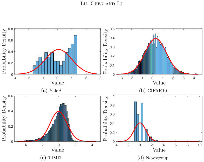
- [Section 2.2 and Figure 16] The real-data validation does not establish the model assumptions. Figure 16 shows marginal histograms of one feature dimension, but the theorems require per-dimension Gaussianity with equal class variances and, for any vector-level extension, independence or a specified dependence structure. The paper does not report how strongly these assumptions are violated on YaleB, TIMIT, Newsgroup, CIFAR10, or ImageNet features, nor whether the enhancing thresholds persist under the measured violations. Without such a check, the generalization from Property 1 to real data remains an assertion.
minor comments (6)
- [Introduction] In the phrase 'In the filed of signal processing,' 'filed' should be 'field.'
- [References] The Charikar reference contains 'thiry-fourth' instead of 'thirty-fourth.'
- [Appendix B.1] In the gradient expression, α = φ(·) and β = φ(·) reuse symbols that were CDFs earlier; these should be written as α′ and β′ or explicitly redefined as densities.
- [Figure 15] The label 'Tenary quantization' in panel (h) should be 'Ternary quantization.'
- [Equation (18)] The term '2aβ' should be '2αβ.'
- [Section 4.2.2] The word 'conductive' in the phrase 'conductive to classification improvement' should be 'conducive.'
Circularity Check
No circular reduction: Theorems 4 and 5 are exact algebraic characterizations, and the real-data experiments are external; the only flagged item is an unproved scalar-to-vector bridge, which is a validity gap rather than circularity.
full rationale
The derivation chain is self-contained. Definition 2 and Definition 3 fix D, Db, and Dt as explicit functions of Gaussian parameters and threshold tau; Theorem 4 and Theorem 5 (with Appendix A) compute closed forms (12), (13), and (18), then solve Db > D and Dt > D into the equivalent inequalities (8) and (9). This is an exact algebraic characterization, not a fitted parameter renamed as a prediction; no empirical constant enters the proof. The numerical validation in Section 3.2 regenerates samples from the same Gaussian model used to derive the formulas, so it verifies arithmetic and sampling consistency rather than providing independent confirmation; that redundancy is not circular because the theorems already stand on the algebra. Real-data experiments in Section 4.2 and Appendix C provide external benchmarks, and the thresholds are searched quantization parameters rather than fitted values that define the discrimination measures. The only self-citation, Lu et al. (2023), is invoked for motivation and for the observation of multiclass improvements, but the current paper's own Figure 20 and real-data results carry that claim, so the citation is not load-bearing. What is genuinely missing is a proof of the Section 2.2 bridge from per-dimension to vector-level discrimination: the statement that vector discrimination 'positively correlates' with element-wise discrimination is an assertion, and the theorems themselves treat scalar dimensions. That is a validity or robustness gap, not a circular reduction, because vector-level discrimination is not defined in terms of element-level discrimination within the derivation. No circular step can be exhibited, so the score is 0.
Assumptions & free parameters
free parameters (1)
- Per-dataset threshold scale γ =
Best value found by scanning test accuracy
assumptions (4)
- domain assumption Two balanced classes drawn from Gaussian distributions with distinct means and equal variance; after standardization, means are symmetric and µ²+σ²=1 (Property 1).
- domain assumption Vector-level discrimination is positively correlated with per-element discrimination, so analysis can be carried out on a single dimension.
- domain assumption Higher Fisher feature discrimination implies easier classification and higher accuracy for KNN and linear SVM.
- domain assumption Real-world features approximately follow per-dimension Gaussian distributions within each class.
Cite this review
Pith. "Pith review of Binary and Ternary Quantization Can Enhance Feature Discrimination." pith.science (2026). https://pith.science/paper/EQPWZLFY
@misc{pith2026250413792,
  author       = {Pith},
  title        = {Pith review of: Binary and Ternary Quantization Can Enhance Feature Discrimination},
  year         = {2026},
  howpublished = {\url{https://pith.science/paper/EQPWZLFY}},
  note         = {Machine review of arXiv:2504.13792}
}
abstract
Quantization is widely applied in machine learning to reduce computational and storage costs for both data and models. Considering that classification tasks are fundamental to the field, it is crucial to investigate how quantization impacts classification performance. Traditional research has focused on quantization errors, assuming that larger errors generally lead to lower classification accuracy. However, this assumption lacks a solid theoretical foundation and often contradicts empirical observations. For example, despite introducing significant errors, $\{0,1\}$-binary and $\{0, \pm1\}$-ternary quantized data have sometimes achieved classification accuracy comparable or even superior to full-precision data. To reasonably explain this phenomenon, a more accurate evaluation of classification performance is required. To achieve this, we propose a direct analysis of the feature discrimination of quantized data, instead of focusing on quantization errors. Our analysis reveals that both binary and ternary quantization can potentially enhance, rather than degrade, the feature discrimination of the original data. This finding is supported by classification experiments conducted on both synthetic and real data.
Figures


Figures from the paper (17 more)




Reference graph
Works this paper leans on
-
[1]
J. S. Baras and S. Dey. Combined compression and classification with learning vector quantization. IEEE Transactions on Information Theory, 45 0 (6): 0 1911--1920, 1999
work page 1911
-
[2]
D. P. Bertsekas. Nonlinear programming. Journal of the Operational Research Society, 48 0 (3): 0 334--334, 1997
1997
-
[3]
M. S. Charikar. Similarity estimation techniques from rounding algorithms. In Proceedings of the thiry-fourth annual ACM symposium on Theory of computing, pages 380--388, 2002
work page 2002
-
[4]
Cortes and V
C. Cortes and V. Vapnik. Support-vector networks. Machine learning, 20 0 (3): 0 273--297, 1995
1995
-
[5]
M. Courbariaux, Y. Bengio, and J.-P. David. Binaryconnect: Training deep neural networks with binary weights during propagations. Advances in neural information processing systems, 28, 2015
work page 2015
-
[6]
S. Dasgupta, C. F. Stevens, and S. Navlakha. A neural algorithm for a fundamental computing problem. Science, 358 0 (6364): 0 793--796, 2017
work page 2017
-
[7]
J. Deng, W. Dong, R. Socher, L.-J. Li, K. Li, and L. Fei-Fei. ImageNet: A Large-Scale Hierarchical Image Database . In IEEE Conference on Computer Vision and Pattern Recognition, 2009
work page 2009
-
[8]
B. M. Dogahe and M. N. Murthi. Quantization for classification accuracy in high-rate quantizers. In Digital Signal Processing and Signal Processing Education Meeting, pages 277--282. IEEE, 2011
work page 2011
Show all 41 references
-
[9]
R. A. Fisher. The use of multiple measurements in taxonomic problems. Annals of eugenics, 7 0 (2): 0 179--188, 1936
1936
-
[10]
W. M. Fisher, G. R. Doddington, and K. M. Goudie-Marshall. The darpa speech recognition research database: Specifications and status. In Proceedings of DARPA Workshop on Speech Recognition, pages 93--99, 1986
1986
-
[11]
Gholami, S
A. Gholami, S. Kim, Z. Dong, Z. Yao, M. W. Mahoney, and K. Keutzer. A survey of quantization methods for efficient neural network inference. In Low-Power Computer Vision, pages 291--326. Chapman and Hall/CRC, 2022
2022
-
[12]
R. M. Gray and D. L. Neuhoff. Quantization. IEEE transactions on information theory, 44 0 (6): 0 2325--2383, 1998
1998
-
[13]
Haufe, R
S. Haufe, R. Tomioka, G. Nolte, K.-R. M \"u ller, and M. Kawanabe. Modeling sparse connectivity between underlying brain sources for EEG/MEG . IEEE transactions on biomedical engineering, 57 0 (8): 0 1954--1963, 2010
1954
-
[14]
K. He, X. Zhang, S. Ren, and J. Sun. Deep residual learning for image recognition. In Proceedings of the IEEE conference on computer vision and pattern recognition, pages 770--778, 2016
2016
-
[15]
Hoefler, D
T. Hoefler, D. Alistarh, T. Ben-Nun, N. Dryden, and A. Peste. Sparsity in deep learning: Pruning and growth for efficient inference and training in neural networks. Journal of Machine Learning Research, 22 0 (241): 0 1--124, 2021
2021
-
[16]
Hutchinson, L
B. Hutchinson, L. Deng, and D. Yu. A deep architecture with bilinear modeling of hidden representations: Applications to phonetic recognition. In IEEE international conference on acoustics, speech and signal processing, pages 4805--4808. IEEE, 2012
2012
-
[17]
Jana and P
S. Jana and P. Moulin. Optimal design of transform coders and quantizers for image classification. In International Conference on Image Processing, volume 3, pages 841--844. IEEE, 2000
2000
-
[18]
Jana and P
S. Jana and P. Moulin. Optimal transform coding of gaussian mixtures for joint classification/reconstruction. In Data Compression Conference, pages 313--322. IEEE, 2003
2003
-
[19]
S. Kotz, T. Kozubowski, and K. Podgorski. The Laplace distribution and generalizations: a revisit with applications to communications, economics, engineering, and finance. Springer Science & Business Media, 2012
2012
-
[20]
Krizhevsky and G
A. Krizhevsky and G. Hinton. Learning multiple layers of features from tiny images. Master's thesis, Department of Computer Science, University of Toronto, 2009
2009
-
[21]
E. Y. Lam and J. W. Goodman. A mathematical analysis of the dct coefficient distributions for images. IEEE transactions on image processing, 9 0 (10): 0 1661--1666, 2000
2000
-
[22]
K. Lang. Newsweeder: Learning to filter netnews. In Machine learning proceedings 1995, pages 331--339. Elsevier, 1995
1995
-
[23]
Larochelle, M
H. Larochelle, M. Mandel, R. Pascanu, and Y. Bengio. Learning algorithms for the classification restricted boltzmann machine. The Journal of Machine Learning Research, 13 0 (1): 0 643--669, 2012
2012
-
[24]
K. Lee, J. Ho, and D. Kriegman. Acquiring linear subspaces for face recognition under variable lighting. IEEE Transactions on Pattern Analysis and Machine Intelligence, 27 0 (5): 0 684--698, 2005
2005
-
[25]
F. Li, B. Zhang, and B. Liu. Ternary weight networks. arXiv, 1605.04711, 2016
2016 arXiv
-
[26]
D. Lin, S. Talathi, and S. Annapureddy. Fixed point quantization of deep convolutional networks. In International conference on machine learning, pages 2849--2858. PMLR, 2016 a
2016
-
[27]
Z. Lin, M. Courbariaux, R. Memisevic, and Y. Bengio. Neural networks with few multiplications. In International Conference on Learning Representations, 2016 b
2016
-
[28]
W. Lu, M. Chen, K. Guo, and W. Li. Quantization: Is it possible to improve classification? In Data Compression Conference, pages 318--327. IEEE, 2023
2023
-
[29]
Mohamed, T
A.-r. Mohamed, T. N. Sainath, G. Dahl, B. Ramabhadran, G. E. Hinton, and M. A. Picheny. Deep belief networks using discriminative features for phone recognition. In IEEE international conference on acoustics, speech and signal processing, pages 5060--5063. IEEE, 2011
2011
-
[30]
K. L. Oehler and R. M. Gray. Combining image compression and classification using vector quantization. IEEE transactions on pattern analysis and machine intelligence, 17 0 (5): 0 461--473, 1995
1995
-
[31]
L. E. Peterson. K-nearest neighbor. Scholarpedia, 4 0 (2): 0 1883, 2009
2009
-
[32]
Poor and J
H. Poor and J. Thomas. Applications of ali-silvey distance measures in the design generalized quantizers for binary decision systems. IEEE Transactions on Communications, 25 0 (9): 0 893--900, 1977
1977
-
[33]
H. Qin, R. Gong, X. Liu, X. Bai, J. Song, and N. Sebe. Binary neural networks: A survey. Pattern Recognition, 105: 0 107281, 2020
2020
-
[34]
J. R. Quinlan. Induction of decision trees. Machine learning, 1: 0 81--106, 1986
1986
-
[35]
D. E. Rumelhart, G. E. Hinton, and R. J. Williams. Learning representations by back-propagating errors. nature, 323 0 (6088): 0 533--536, 1986
1986
-
[36]
Simonyan and A
K. Simonyan and A. Zisserman. Very deep convolutional networks for large-scale image recognition. arXiv preprint arXiv:1409.1556, 2014
2014 arXiv
-
[37]
Srinivasamurthy and A
N. Srinivasamurthy and A. Ortega. Reduced complexity quantization under classification constraints. In Data Compression Conference, pages 402--411. IEEE, 2002
2002
-
[38]
Torralba and A
A. Torralba and A. Oliva. Statistics of natural image categories. Network: computation in neural systems, 14 0 (3): 0 391--412, 2003
2003
-
[39]
M. J. Wainwright and E. P. Simoncelli. Scale mixtures of gaussians and the statistics of natural images. In Proceedings of the 12th International Conference on Neural Information Processing Systems, 1999
1999
-
[40]
H. Wang, S. Ma, L. Dong, S. Huang, H. Wang, L. Ma, F. Yang, R. Wang, Y. Wu, and F. Wei. Bitnet: Scaling 1-bit transformers for large language models. arXiv preprint arXiv:2310.11453, 2023
2023 arXiv
-
[41]
Weiss and W
Y. Weiss and W. T. Freeman. What makes a good model of natural images? In IEEE Conference on Computer Vision and Pattern Recognition, pages 1--8. IEEE, 2007
2007
Reviewed August 16, 2026 · model on record in the stance chip above.
Discussion (0). Continue with ORCID to comment.