Tuning the nonlinear dispersive coupling of nanomechanical string resonators

E. M. Weig; G. Rastelli; K. Gajo

REVIEW 3 major objections 6 minor 18 references

Tuning the nonlinear dispersive coupling of nanomechanical string resonators

T0 review · 3 major / 6 minor · reviewed 2026-08-14 · deepseek-v4-flash

Challenge this review Re-run · record.json Download PDF Read on arXiv ↗ Review JSON

Pith's one-line read This paper shows that the nonlinear dispersive coupling between flexural modes of nanomechanical string resonators is governed by the DC-voltage-dependent hybridization of the bare modes, providing a route to electrically tune nonlinear…

desk verdict A credible experimental first for nonlinear dispersive coupling between two distinct nanomechanical strings, with a nice hybridization model that currently has a factor-of-2 derivation error and only qualitative validation. read the letter →

arxiv 1908.01299 v2 pith:EUSWTB2J submitted 2019-08-04 cond-mat.mes-hall

K. Gajo , G. Rastelli , E. M. Weig This is my paper · ORCID

classification cond-mat.mes-hall

keywords nanomechanicalresonatorsnonlinearmodecouplingdispersiveDuffingnonlinearityhybridizationavoidedcrossingsdielectrictuningsiliconnitridestrings

verification ladder T0 review T1 audit T2 compute T3 formal

The pith

A machine-rendered reading of the paper's core claim, the machinery that carries it, and where it could break.

The reading

The paper investigates two doubly clamped silicon nitride string resonators whose flexural modes hybridize because of a shared clamping point and a DC-voltage-controlled dielectric force. When one hybridized eigenmode is driven into its nonlinear regime, the other two eigenmodes shift in frequency, revealing nonlinear dispersive coupling between them. The central claim is that the voltage dependence of both the Duffing nonlinearity and the dispersive coupling coefficients is carried by the voltage-dependent hybridization of the bare modes, described by explicit formulas relating hybridized and bare nonlinear coefficients. The paper demonstrates the effect experimentally and shows that its model reproduces the observed voltage dependence qualitatively, while noting that a quantitative check requires calibrated displacement detection.

What carries the argument

The load-bearing object is the mode-hybridization matrix $e_{ji}(U_{\mathrm{dc}})$, the eigenvectors of the linear mode matrix $\Theta$ that diagonalizes the three coupled bare modes. The transformation $v_i = \sum_j e_{ji} q_j$ moves from bare amplitudes to hybridized eigenmode amplitudes, and the quartic potential of Eq. (11) becomes Eq. (12); discarding cubic and three-body terms far from internal resonances leaves effective Duffing and dispersive terms. Eqs. (13) and (14) then express $\tilde{\gamma}_{ii}$ and $\tilde{\gamma}_{ij}$ as sums of bare coefficients $\gamma_{jk}$ multiplied by products of four eigenvector entries. All voltage dependence of the nonlinear coefficients enters through these eigenvector products, which is the mechanism the paper uses to explain the measured voltage dependence.

What would settle it

Drive a pair of hybridized modes whose eigenvector composition is essentially constant as the DC voltage is varied (for example, well away from all avoided crossings) and measure the dispersive coupling between them; if the coupling changes appreciably with voltage, the bare nonlinear coefficients themselves are voltage-dependent and the hybridization-only model is incomplete. Alternatively, a fully calibrated displacement measurement that removes the unknown factors $c_i$ would reveal whether the predicted quantitative voltage curves match the data.

Watch

Extended reading notes

Core claim

The central discovery is that in a system of linearly coupled mechanical modes, the nonlinear coefficients of the hybridized eigenmodes are not fixed properties of the resonators but functions of the eigenvector matrix that encodes the mode polarization. By writing the quartic potential of the bare modes in the hybridized basis, the paper obtains closed expressions, Eqs. (13) and (14), in which the Duffing nonlinearity $\tilde{\gamma}_{ii}$ and the dispersive coupling $\tilde{\gamma}_{ij}$ of the eigenmodes are linear combinations of the bare-mode nonlinearities $\gamma_{ij}$, weighted by products of four eigenvector components. Since the eigenvectors depend on the DC voltage through the avoided crossings, the nonlinear coefficients inherit a voltage dependence. Experimentally, driving the intermediate eigenmode produces clear frequency shifts of the two other eigenmodes, and the extracted coefficients vary strongly with voltage, especially near the avoided crossings. The paper claims that the model captures the qualitative features of this variation, supporting the interpretation that hybridization controls the nonlinear coupling.

Load-bearing premise

The argument assumes that the intrinsic nonlinear coefficients of the bare modes are independent of the DC voltage, so that all measured voltage dependence of the effective nonlinearities comes from the changing mode hybridization; the paper itself flags that a voltage-dependent dielectric modulation of the bare nonlinearities would also produce such a dependence.

Editorial extensions

If this is right

A DC voltage becomes a continuous control knob for the effective Duffing nonlinearity and the dispersive coupling of each hybridized mode, not just for its frequency.
Near multimode avoided crossings, the dispersive coupling coefficients can change magnitude and sign as bare-mode weights are redistributed, so the same device can be switched between different nonlinear interaction regimes.
The model gives a predictive recipe: from a linear fit of the eigenfrequencies one obtains the eigenvectors, and with a few bare-mode nonlinear parameters one can forecast the voltage dependence of all nonlinear coefficients.
The observed amplitude-induced frequency shifts of two undriven modes demonstrate that dispersive coupling persists even far from internal resonances, an effect that could be used for mode-selective sensing or signal processing.
For nanomechanical networks, the result implies that nonlinear responses can be electrically reprogrammed by tuning hybridization, without changing the physical geometry.

Reading between the lines

Editorial extensions of the paper, not claims the author makes directly.

If the same eigenvector-weighting rule applies beyond mechanics, then in any network of linearly coupled nonlinear oscillators (electrical or optical) the nonlinear couplings can be tuned by the same linear mode mixing, so the mechanism is a general design principle.
The paper leaves open whether the bare-mode nonlinear coefficients themselves change with voltage; if they do, the observed curves are a convolution of hybridization with direct dielectric modulation, and a clean separation could be made by measuring a pair of modes that never hybridize.
A fully calibrated detection scheme would turn the model into a spectroscopic tool: fitting the voltage-dependent curves would extract the bare nonlinear coefficients $\gamma_{ij}$, which are otherwise hard to access directly.
Near internal resonances, the discarded cubic and three-body terms in Eq. (12) would become active, so the same system should display additional nonlinear effects such as energy exchange and combination resonances; probing those would test the validity of the far-from-resonance approximation.

Share X Bluesky LinkedIn Reddit HN

Signed reviews

No signed human review yet.

Editorial analysis

A structured set of objections, weighed in public.

Desk editor's note, referee report, and a circularity audit.

Desk Editor's Note

read the letter

Two things to know. First, this is a legitimate experimental first: nonlinear dispersive coupling between two distinct, elastically coupled nanomechanical resonators, not just between modes of one resonator. The frequency-shift data in Fig. 4 are believable and clearly show the effect. Second, the theoretical model advertised as showing how the coupling inherits the voltage-tuned hybridization has a concrete internal inconsistency: Eq. (14) does not follow from Eqs. (11)-(12). Direct substitution gives a factor of 2 smaller coefficient for the gamma_kk terms. The paper is still worth a serious referee, but the derivation needs fixing.

What is actually new is the demonstration that the dispersive coupling and the Duffing coefficient depend on the mode hybridization in a two-string system, and the simple basis-transformation picture. The model is an independent prediction: the eigenvector components come from a genetic fit to the linear avoided-crossing data, and the nonlinear measurements are not used to set the bare gamma parameters. So the circularity burden is low. The citation list covers the prior work; the claim that earlier demonstrations were within individual resonators holds up. The authors also deserve credit for being upfront in Sec. VI about the uncalibrated detection factors and the possibility that the bare gamma_ij themselves depend on DC voltage — the latter is flagged as a missing ingredient.

Soft spots, in proportion. The factor-of-2 issue is the most concrete. Using the definition in Eq. (12), the q_i^2 q_j^2 coefficient from 1/4 gamma_kk v_k^4 is (3/2) gamma_kk e_ik^2 e_jk^2, which gives tilde_gamma_ij = 3 sum_k ..., not 6. Unless Eq. (12) is misprinted, the quantitative curves in Fig. 6 are off by a constant factor. Since the comparison is qualitative only, this does not sink the qualitative claim, but the model as written is not well defined. Second, the experimental validation is limited: the extracted tilde c_i tilde gamma_ij are uncalibrated, have no error bars, and the comparison with theory is visual. The hand-picked bare gamma values (e.g., gamma_33/gamma0 = 0.01) make the theoretical curves illustrative rather than predictive. These limitations are acknowledged in the paper.

Who should read it: people working on coupled nanomechanical systems or nonlinear mode-coupling. The experiment itself is a solid addition. The model should be corrected before anyone relies on the quantitative form; the qualitative picture is probably right.

Recommendation: send it to peer review. A referee should ask for the Eq. (14) derivation to be redone, the prefactor clarified, and a quantitative comparison once calibration is available — but the work deserves that round.

Referee Report

3 major / 6 minor

Summary. This manuscript reports an experimental study of nonlinear dispersive coupling among the three lowest hybridized flexural modes of a pair of nanomechanical silicon-nitride string resonators. A drive tone is swept through one eigenmode while the thermally activated frequencies of the other two eigenmodes are monitored; the observed amplitude-dependent shifts are fitted to extract voltage-dependent Duffing and dispersive-coupling coefficients. The authors then introduce a model in which the bare modes and their quartic nonlinearities are projected onto the voltage-dependent eigenmodes of the linear coupling matrix, yielding predicted voltage dependences of the hybridized nonlinear coefficients. The comparison between theory and experiment is qualitative, as the detection calibration factors and some bare nonlinear parameters are not independently determined.

Significance. The conceptual contribution is potentially useful: it gives a transparent mechanism, mode hybridization, through which electrostatic tuning can alter the nonlinear coefficients of a multimode nanomechanical system. The direct observation of nonlinear dispersive frequency shifts in a strongly coupled three-mode system is also of experimental interest. The paper is explicit about the main limitations, namely unknown calibration factors, hand-chosen bare nonlinear parameters, and the possible voltage dependence of the bare nonlinearities. However, the central quantitative formula contains a factor-of-two algebraic error, and the experimental data cannot currently constrain the model at a quantitative level. With a corrected derivation and a more stringent comparison, the paper would be a solid contribution.

major comments (3)

[VI, Eq. (14)] Equation (14) does not follow from substituting Eq. (5) into Eq. (11) with the convention of Eq. (12). For the diagonal terms, the q_i^2 q_j^2 coefficient coming from (1/4) sum_k gamma_kk v_k^4 is (3/2) sum_k gamma_kk e_ik^2 e_jk^2, whereas Eq. (12) writes the cross term as (1/2) tilde_gamma_ij q_i^2 q_j^2. Equating these gives tilde_gamma_ij = 3 sum_k gamma_kk e_ik^2 e_jk^2, not the factor 6 appearing in Eq. (14). The gamma_km terms in Eq. (14) are overcounted by the same factor of two; for ordered sums over k != m the corrected expression is tilde_gamma_ij = 3 sum_k e_ik^2 e_jk^2 gamma_kk + (1/2) sum_{k != m} (e_ik^2 e_jm^2 + e_jk^2 e_im^2) gamma_km + 2 sum_{k != m} e_ik e_jm e_jk e_im gamma_km, with i != j. Unless a different prefactor convention in Eq. (12) is intended and explicitly stated, the curves in Fig. 6 are a factor of two too large. This is a load-bearing error because Eq. (14) is the quantitative content of the central model.
[VI, Fig. 6 and final paragraphs] The bare nonlinear parameters gamma_ij used in Fig. 6 are chosen by hand as 'realistic' values and are not constrained by the measured nonlinear coefficients, and no uncertainty is given for them. The experiment measures only products c_i tilde_gamma_ij with unknown, possibly voltage-dependent calibration factors c_i; the manuscript explicitly states that these factors could not be extracted and that the voltage dependence of the bare gamma_ij is not included in the model. These are appropriate caveats, but they mean the experimental data cannot quantitatively validate Eqs. (13) and (14). The observed voltage dependence could, for example, originate from dielectric modulation of the bare nonlinearities rather than from hybridization. I do not regard this as an internal inconsistency, but it does limit the strength of the central claim. The authors should either provide a calibration-independent observable derived from the model or fit the bare gamma_ij to the measured voltage-dependent coefficients and show residuals.
[IV, Eqs. (9)-(10)] The extracted coefficients c2 tilde_gamma_12 and c2 tilde_gamma_23 are given with four significant digits but with no uncertainties and without a discussion of how the linear fits were weighted. Since Fig. 5 presents these values as the main experimental result of the voltage-dependence study, the absence of error bars makes it difficult to judge whether the apparent voltage dependence is statistically significant and whether the qualitative agreement claimed in Section VI is meaningful.

minor comments (6)

[III, Fig. 3 caption] The word 'bue' should be 'blue', and 'eingenmode' should be 'eigenmode'; similar typos appear elsewhere, including 'Moreveover' in Section VI.
[I, Eq. (1)] The sum written as sum_{i != j} gamma_ij v_j^2 inside the equation for v_i uses the index i in the summation symbol; it should be sum_{j != i} gamma_ij v_j^2.
[VI, Eqs. (13)-(14)] The eigenvector index convention is confusing: Eq. (5) defines v_i = sum_j e_ji q_j, while Eqs. (13)-(14) and Fig. 3 use e_ij with the indices apparently reversed. The matrix e should be defined explicitly as the matrix whose columns or rows are the eigenvectors of Theta.
[V, Fig. 5] The axes and data points in Fig. 5 would benefit from error bars and from an explicit statement of the units of the plotted products c_i tilde_gamma_ij and c_i tilde_gamma_ii.
[VI, Eq. (12)] The coefficients psi_ij and phi_i in Eq. (12) are not defined; even if these terms are subsequently neglected, a sentence explaining their origin and order of magnitude would help the reader.
[References] Reference [8] has a corrupted author field ('A. and-Patton'); the bibliographic data should be checked against the published record.

Circularity Check

0 steps flagged · score 2.0 of 10

No significant circularity: the hybridization-dependent nonlinear coefficients are derived algebraically from a quartic potential and linear-fit eigenvectors, with nonlinear data not used to set model parameters.

full rationale

The paper's central claim—that the Duffing nonlinearity and dispersive coupling depend on mode hybridization—follows from substituting the eigenvector expansion Eq. (5) into the fourth-order potential Eq. (11), yielding Eqs. (13)–(14). The eigenvectors e_ij(Vdc) come from a genetic fit to the linear frequency data of Fig. 2, and the six bare gamma parameters used for Fig. 6 are explicitly labeled 'realistic parameters,' not fitted to the measured nonlinear frequency shifts. The measured quantities are c_i*gamma_ij with unknown, voltage-dependent calibration factors, so the paper itself says the comparison is qualitative. Therefore no measured nonlinear quantity is used as an input to compute the predicted curves; the predicted voltage dependence is not forced by construction. The only self-citation [10] supplies the shared-clamp linear coupling and the genetic-fit method; it is methodological and not load-bearing for the nonlinear prediction, and no uniqueness theorem from the authors is invoked. Section VI explicitly acknowledges that the bare gamma_ij may themselves depend on Udc and that calibration is incomplete; this is a stated limitation, not a circular step. Even if Eq. (14) contains an algebraic factor-of-2 inconsistency, as the skeptic claims, that is an internal correctness issue, not circularity.

Assumptions & free parameters 20 free parameters · 6 assumptions · 0 invented entities

The central nonlinear claim rests on the linear fit parameters through the eigenvector matrix and on six bare nonlinear coefficients that are chosen by hand and not measured. The model is not circular in using the nonlinear data to set these parameters, but its predictive strength is limited by the unmeasured calibration factors and by the assumed voltage independence of the bare coefficients.

free parameters (20)

kappa12/(2pi)^2 = 4.138 MHz^2
Linear coupling between OP1 and OP2, fitted to the avoided crossings in Fig. 2; enters the eigenvector matrix used by the nonlinear model.
kappa13/(2pi)^2 = 1.9098 MHz^2
Linear coupling between OP1 and IP1 from the genetic fit in Section III.
kappa23/(2pi)^2 = 2.546 MHz^2
Linear coupling between OP2 and IP1 from the genetic fit in Section III.
omega10/(2pi) = 5.8606 MHz
Bare OP1 frequency at zero voltage and zero coupling from the fit.
omega20/(2pi) = 5.9897 MHz
Bare OP2 frequency at zero voltage and zero coupling from the fit.
omega30/(2pi) = 6.1117 MHz
Bare IP1 frequency at zero voltage and zero coupling from the fit.
U10 = 0.656 V
Voltage offset for the OP1 tuning parabola, fitted in Section III.
U20 = -1.1 V
Voltage offset for the OP2 tuning parabola, fitted in Section III.
U30 = 0.485 V
Voltage offset for the IP1 tuning parabola, fitted in Section III.
c1/(2pi) = 165.59 Hz/V^2
Quadratic voltage tuning coefficient for OP1, fitted in Section III.
c2/(2pi) = 1 Hz/V^2
Quadratic voltage tuning coefficient for OP2, fitted in Section III.
c3/(2pi) = -282.5 Hz/V^2
Quadratic voltage tuning coefficient for IP1, fitted in Section III.
d1/(2pi) = 1.368 Hz/V^3
Cubic voltage tuning correction for OP1, fitted in Section III.
d3/(2pi) = -2.2 Hz/V^3
Cubic voltage tuning correction for IP1, fitted in Section III.
gamma11/gamma0 = 2.2
Bare Duffing coefficient for OP1, chosen as a realistic parameter for the illustrative model in Section VI; not measured or independently derived.
gamma22/gamma0 = 3.8
Bare Duffing coefficient for OP2, chosen as a realistic parameter for the illustrative model in Section VI.
gamma33/gamma0 = 0.01
Bare Duffing coefficient for IP1, chosen as a realistic parameter for the illustrative model in Section VI.
gamma12/gamma0 = -6.5
Bare dispersive coupling between OP1 and OP2, chosen as a realistic parameter for the illustrative model in Section VI.
gamma13/gamma0 = 0.8
Bare dispersive coupling between OP1 and IP1, chosen as a realistic parameter for the illustrative model in Section VI.
gamma23/gamma0 = 1.3
Bare dispersive coupling between OP2 and IP1, chosen as a realistic parameter for the illustrative model in Section VI.

assumptions (6)

domain assumption The system can be described by three linearly coupled, weakly nonlinear harmonic oscillators with a quartic potential (Eqs. 1 and 11).
The string modes are treated as lumped oscillators with Duffing and dispersive terms; damping, drive, and noise are omitted from the derivation of Eqs. (13) and (14).
domain assumption The linear coupling constants kappa_ij are independent of DC voltage, neglecting dielectric effects on the coupling.
Stated in Section III before Eq. (3); if false, the eigenvector basis used to transform the nonlinear terms is voltage-distorted.
domain assumption The eigenfrequency tuning curves are quadratic with cubic corrections: omega_i(Udc) = omega_i0 + c_i (Udc - U_i0)^2 + d_i (Udc - U_i0)^3.
A phenomenological choice fitted to the data in Section III; no microscopic derivation is given.
domain assumption The intrinsic nonlinear coefficients gamma_ij of the bare modes are independent of DC voltage.
Acknowledged in Section VI as not included in the model; if false, observed voltage dependence could come from intrinsic dielectric modulation rather than hybridization.
domain assumption Cubic and three-body terms appearing in the transformed potential (Eq. 12) can be neglected because the drive is single-frequency and far from internal resonances.
Standard secular approximation, stated in Section VI.
standard math The eigenvectors e_ji(Vdc) from the linear fit form an orthogonal matrix, so the inverse transform equals the transpose.
Theta in Eq. (4) is symmetric, so its eigenvectors are orthogonal after normalization.

how reviews work

0 comments

Cite this review

Pith. "Pith review of Tuning the nonlinear dispersive coupling of nanomechanical string resonators." pith.science (2026). https://pith.science/paper/EUSWTB2J

@misc{pith2026190801299,
  author       = {Pith},
  title        = {Pith review of: Tuning the nonlinear dispersive coupling of nanomechanical string resonators},
  year         = {2026},
  howpublished = {\url{https://pith.science/paper/EUSWTB2J}},
  note         = {Machine review of arXiv:1908.01299}
}

read the original abstract

We investigate nonlinear dispersive mode coupling between the flexural in- and out-of-plane modes of two doubly clamped, nanomechanical silicon nitride string resonators. As the amplitude of one mode transitions from the linear response regime into the nonlinear regime, we find a frequency shift of two other modes. The resonators are strongly elastically coupled via a shared clamping point and can be tuned in and out of resonance dielectrically, giving rise to multimode avoided crossings. When the modes start hybridizing, their polarization changes. This affects the nonlinear dispersive coupling in a non-trivial way. We propose a theoretical model to describe the dependence of the dispersive coupling on the mode hybridization.

Figures

Figures reproduced from arXiv: 1908.01299 by the authors.

**Figure 2.** FIG. 2. (color online) Frequency response of hybridized [PITH_FULL_IMAGE:figures/full_fig_p002_2.png] view at source ↗

**Figure 3.** FIG. 3. (color online) a) Frequencies of the hybridized eigen [PITH_FULL_IMAGE:figures/full_fig_p003_3.png] view at source ↗

Figures from the paper (2 more)

**Figure 4.** Figure 4: FIG. 4. (color online) a) Power spectra for varying drive [PITH_FULL_IMAGE:figures/full_fig_p004_4.png]

**Figure 5.** Figure 5: FIG. 5. (color online) Nonlinear coefficients (including mode [PITH_FULL_IMAGE:figures/full_fig_p004_5.png]

Discussion (0). Continue with ORCID to comment.

Reference graph

Works this paper leans on

18 extracted references · 16 canonical work pages

[1]

This mode has the strongest contribution from the bare mode OP2 (see Fig

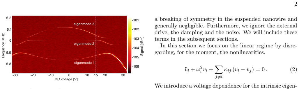
On the other hand, mode 2 is almost ﬂat. This mode has the strongest contribution from the bare mode OP2 (see Fig. 3c), which is only indirectly aﬀected by the tun- ing of resonator 1. Finally, the bare modes strongly hybridize in the area of the avoided crossings between 15 V and 28 V. Note that the microwave cavity-assisted readout technique is sensi- t...

work page
[2]

Figures 4c and 4d show the shift of the frequencies ˜Ω2 1 of eigenmode 1 (blue dots) and ˜Ω2 3 of eigenmode 3 (green dots) as a function of the amplitude of the driven eigen- mode

(10) As mentioned above, the dispersive coupling manifests itself in a frequency shift of one mode, if the vibration amplitude of another mode is changed. Figures 4c and 4d show the shift of the frequencies ˜Ω2 1 of eigenmode 1 (blue dots) and ˜Ω2 3 of eigenmode 3 (green dots) as a function of the amplitude of the driven eigen- mode. We carry out a ﬁt of ...

work page 2020
[3]

Mangussi and D

F. Mangussi and D. H. Zanette, PLOS ONE11, e0162365 (2016)

work page 2016
[4]

Vinante, Phys

A. Vinante, Phys. Rev. B 90, 024308 (2014)

work page 2014
[5]

H. J. R. Westra, M. Poot, H. S. J. van der Zant, and W. J. Venstra, Phys. Rev. Lett. 105, 117205 (2010)

work page 2010
[6]

van der Avoort, R

C. van der Avoort, R. van der Hout, J. J. M. Bontemps, P. G. Steeneken, K. L. Phan, R. H. B. Fey, J. Hulshof, and J. T. M. van Beek, J. of Micromech. and Microen. 20, 105012 (2010)

work page 2010
[7]

K. J. Lulla, R. B. Cousins, M. J. Venkatesan, A. and- Patton, A. D. Armour, C. J. Mellor, and J. R. Owers- Bradley, New J. Phys. 14, 113040 (2012)

work page 2012
[8]

M. H. Matheny, L. G. Villanueva, R. B. Karabalin, J. E. Sader, and M. L. Roukes, Nano Lett. 13, 1622 (2013)

work page 2013

Show all 18 references

[9]

Cadeddu, F

D. Cadeddu, F. R. Braakman, G. T¨ ut¨ unc¨ uoglu, F. Mat- teini, D. R¨ uﬀer, A. Fontcuberta i Morral, and M. Poggio, Nano Lett. 16, 926 (2016)

2016
[10]

X. Dong, M. I. Dykman, and H. B. Chan, Nat. Comm. 9, 3241 (2018)

2018
[11]

J. P. Mathew, A. Bhushan, and M. M. Deshmukh, Sol. State Comm. 282, 17 (2018)

2018
[12]

K. Gajo, S. Sch¨ uz, and E. M. Weig, Appl. Phys. Lett. 111, 133109 (2017)

2017
[13]

Q. P. Unterreithmeier, E. M. Weig, and J. P. Kotthaus, Nature 458, 1001 (2009)

2009
[14]

Rieger, T

J. Rieger, T. Faust, M. J. Seitner, J. P. Kotthaus, and E. M. Weig, Appl. Phy. Lett. 101, 103110 (2012)

2012
[15]

Faust, P

T. Faust, P. Krenn, S. Manus, J. P. Kotthaus, and E. M. Weig, Nat. Comm. 3, 728 (2012)

2012
[16]

J. S. Huber, G. Rastelli, M. J. Seitner, J. K¨ olbl, W. Belzig, M. I. Dykman, and E. M. Weig, e-prints , arXiv:1903.07601 (2019), 1903.07601

2019 arXiv
[17]

Zhang and M

Y. Zhang and M. I. Dykman, Phys. Rev. B 92, 165419 (2015)

2015
[18]

Singh, A

R. Singh, A. Sarkar, C. Guria, R. Nicholl, S. Chakraborty, K. I. Bolotin, and S. Ghosh, eprint arXiv:1904.01613 (2019)

2019 arXiv

Pith tools

Reviewed August 14, 2026 · model on record in the stance chip above.

[1] [1]

This mode has the strongest contribution from the bare mode OP2 (see Fig

On the other hand, mode 2 is almost ﬂat. This mode has the strongest contribution from the bare mode OP2 (see Fig. 3c), which is only indirectly aﬀected by the tun- ing of resonator 1. Finally, the bare modes strongly hybridize in the area of the avoided crossings between 15 V and 28 V. Note that the microwave cavity-assisted readout technique is sensi- t...

work page

[2] [2]

Figures 4c and 4d show the shift of the frequencies ˜Ω2 1 of eigenmode 1 (blue dots) and ˜Ω2 3 of eigenmode 3 (green dots) as a function of the amplitude of the driven eigen- mode

(10) As mentioned above, the dispersive coupling manifests itself in a frequency shift of one mode, if the vibration amplitude of another mode is changed. Figures 4c and 4d show the shift of the frequencies ˜Ω2 1 of eigenmode 1 (blue dots) and ˜Ω2 3 of eigenmode 3 (green dots) as a function of the amplitude of the driven eigen- mode. We carry out a ﬁt of ...

work page 2020

[3] [3]

Mangussi and D

F. Mangussi and D. H. Zanette, PLOS ONE11, e0162365 (2016)

work page 2016

[4] [4]

Vinante, Phys

A. Vinante, Phys. Rev. B 90, 024308 (2014)

work page 2014

[5] [5]

H. J. R. Westra, M. Poot, H. S. J. van der Zant, and W. J. Venstra, Phys. Rev. Lett. 105, 117205 (2010)

work page 2010

[6] [6]

van der Avoort, R

C. van der Avoort, R. van der Hout, J. J. M. Bontemps, P. G. Steeneken, K. L. Phan, R. H. B. Fey, J. Hulshof, and J. T. M. van Beek, J. of Micromech. and Microen. 20, 105012 (2010)

work page 2010

[7] [7]

K. J. Lulla, R. B. Cousins, M. J. Venkatesan, A. and- Patton, A. D. Armour, C. J. Mellor, and J. R. Owers- Bradley, New J. Phys. 14, 113040 (2012)

work page 2012

[8] [8]

M. H. Matheny, L. G. Villanueva, R. B. Karabalin, J. E. Sader, and M. L. Roukes, Nano Lett. 13, 1622 (2013)

work page 2013