REVIEW 3 major objections 6 minor 34 references
A convolutional neural network can recover two-dimensional velocity-delay maps from reverberation mapping data, even when the light curves are noisy and have gaps.
Reviewed by Pith at T0; open to challenge. T0 means a machine referee read the full paper against a public rubric. the ladder, T0–T4 →
T0 review · deepseek-v4-flash
2026-08-03 13:20 UTC pith:EYLGOE5U
load-bearing objection A useful within-subfield methods paper that shows a CNN ensemble can deconvolve RM data well inside the training distribution, but generalization to real data is not yet demonstrated — and the paper is honest about that. the 3 major comments →
A Convolutional Neural Network for the Recovery of Transfer Functions From Velocity-Resolved Reverberation Mapping Data
The pith
A machine-rendered reading of the paper's core claim, the machinery that carries it, and where it could break.
Core claim
The central claim is that the reverberation-mapping deconvolution problem—recovering the response function Ψ(ν, τ) from noisy, gappy line and continuum light curves—can be solved by a convolutional network that learns the operator f(ΔC) such that Ψ = f(ΔC)*ΔL. Trained on tens of thousands of synthetic examples built from damped random walk continua and a library of ring, Gaussian, exponential, disk, cloud, and disk-wind response shapes, the network generalizes to unseen transfer functions, degrades gracefully when observations are missing, and produces uncertainty estimates from an ensemble. The authors demonstrate 1D and 2D recoveries, transfer learning to a different continuum, and agreeme
What carries the argument
The central object is the (D)CNN architecture, a convolutional network with three parallel branches of small, medium, and large temporal and velocity filters, followed by a skip-connection chain and a 1×1 convolution to output the map. It is built on the identity that the inverse operator in the convolution theorem can be learned as a data-driven function f(ΔC) which, convolved with the line light curve, yields the transfer function. Training uses a synthetic data pipeline: a damped-random-walk continuum, transfer functions drawn from three families of shapes plus additive combinations, 0.5% white noise, and randomly dropped data points. The ensemble of ~20–40 networks supplies empirical err
Load-bearing premise
The method's validity rests on the assumption that synthetic training data—generated by convolving a damped random walk continuum with a library of hand-built transfer functions, adding 0.5% white noise and random gaps, and assuming perfectly de-trended, continuum-free light curves—are representative enough of real reverberation mapping data that a network trained on them will recover true transfer functions from observations.
What would settle it
Feed the trained ensemble a set of light curves from a real AGN whose velocity-delay response has been independently mapped by a fully physical model (e.g., one with sharp edges and a red-blue asymmetry), and check whether the ensemble's 1σ recovery region contains that independent map. If it does not, or if the spurious prompt-response artifact seen in the paper's blind test persists after continuum contamination is added to the training set as the authors propose, the method's generalization claim would be falsified.
If this is right
- If correct, the method offers a cheap, fast alternative to regularized inversion codes for producing velocity-delay maps from current and future 2D reverberation campaigns, with uncertainties computed directly from the ensemble.
- The method could be applied to any reverberation deconvolution problem, including accretion disk and torus reverberation mapping, not just the broad-line region.
- Because transfer learning requires only a few epochs to adapt to a new continuum, the same trained ensemble can be fine-tuned for individual sources, easing the analysis burden expected from upcoming survey data.
- The blind test demonstrates that the recovered maps agree with existing analytic inversions, suggesting the method can be used as a cross-check on those results.
- The failure mode identified in the blind test—spurious prompt response due to continuum contamination—points to a concrete improvement: adding continuum contamination to the training set would likely resolve it.
Where Pith is reading between the lines
- Editorial inference: The authors' own interpretability tests suggest the multi-scale split architecture may be unnecessary; a simpler skip-only network might perform equally well and be faster to train, a direction they explicitly flag for future work.
- Editorial inference: Because the method depends on the assumed linear convolution model, it will likely inherit systematics from nonlinear or time-varying response behavior; a testable extension is probing recovery on simulations with nonlinear line response.
- Editorial inference: Since the training set excludes continuum contamination, real-data applications with imperfect continuum subtraction will tend to produce spurious prompt response (as in the blind test); a practical workaround is co-training with contaminated light curves, which the paper suggests for the future.
- Editorial inference: The ensemble uncertainty estimates appear calibrated on synthetic data, but a stronger reliability test would apply the method to a source with an independent geometric or dynamical model and compare the recovered map directly.
Editorial analysis
A structured set of objections, weighed in public.
Referee Report
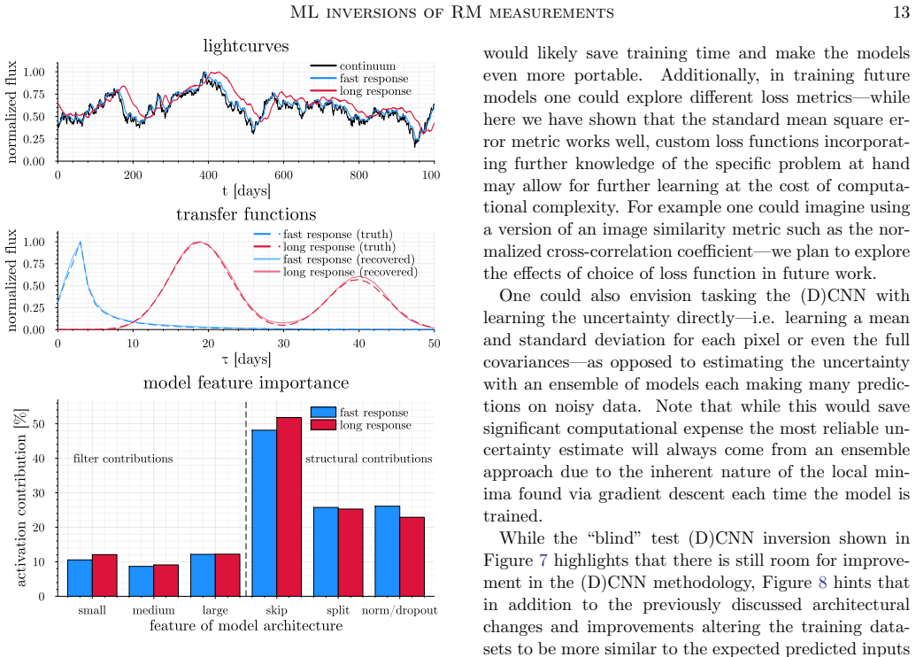
Summary. This manuscript presents a convolutional neural network ensemble for recovering the one- and two-dimensional transfer functions (velocity-delay maps) from synthetic reverberation-mapping light curves. The network is trained on mock line light curves produced by convolving a single DRW continuum with a mixture of analytic basis shapes, an accretion-disk prescription, and kinematic BLR models, with white noise and randomized gaps. On held-out synthetic data from the same generator the method recovers 1D and 2D transfer functions accurately, degrades gracefully with 10–50% missing data, produces ensemble uncertainties that visually track residuals, and compares favorably with MEMEcho. Transfer learning to a different continuum is demonstrated, and a blind test on Mangham et al. synthetic spectra reproduces the main velocity-delay structure but adds a spurious prompt-response component, which the authors attribute to continuum contamination absent from training. Interpretability experiments show that the physically motivated scale-split filters do not activate in the expected way.
Significance. The in-distribution results are credible, and the combination of a simple CNN architecture with an ensemble for uncertainty estimation is a useful practical contribution for RM analysis. The reproducibility assets (code and sample models) are a positive feature. However, the broad claim that the method 'can successfully deconvolve reverberation mapping data products' is not yet established for real or out-of-distribution data, and the key conceptual limitation that the continuum is not an input to the network needs to be addressed or prominently disclosed. If these points are fixed, the paper would be a solid methods contribution to the RM community.
major comments (3)
- [§2.1–2.2, Eq. (1)–(3)] The network input is the line light curve/spectrogram alone; the continuum is used only to generate the training data. Thus the learned map is not the general inverse f(ΔC) in Eq. (3), but a supervised regression from ΔL to Ψ that is conditional on the specific DRW continuum used in training and on the hand-built Ψ families. The paper acknowledges this in §5, but the abstract and §7 statements that the method can 'successfully deconvolve reverberation mapping data products' and could be applied to 'any reverberation deconvolution problem' overstate the current evidence. Please qualify these claims, e.g., by describing the method as a continuum-conditioned supervised inversion rather than a general deconvolution.
- [§5, Fig. 7] The only out-of-family blind test shows a systematic artifact: extra prompt response at τ≈0 that is not present in the MEMEcho recovery. The authors' explanation (continuum contamination absent from the training set) is plausible, but it means the method has not been validated on the type of input it will encounter in real RM data. All quantitative successes in Figs. 2–6 are generated by the same pipeline used for training. I recommend adding a test in which continuum contamination is included in the training set, or carrying out a more aggressive continuum-subtraction step and showing that the artifact is removed, or explicitly restricting the central claim to in-distribution synthetic data.
- [§3.1, §4, Fig. 5d] The claims that 'the error bar always encapsulates the true response function' and that confidence intervals are 'sensible' are based on visual inspection of in-distribution validation examples. No coverage fraction is reported, and the blind test in Fig. 7 does not compare the predicted uncertainty map to the true residual. Because the ensemble spread accounts for training and input noise but not systematic errors from distribution shift, the uncertainty should be presented as conditional on the training distribution unless a quantitative coverage test on out-of-distribution data is added.
minor comments (6)
- [§2.2/References] Horne et al. 1991a and 1991b are listed as separate references but appear to be the same paper (ApJL 367, L5). Please correct the citation.
- [§2.2] All training transfer functions are normalized, so the method predicts only the shape of Ψ, not its absolute responsivity. This is an important limitation and should be stated in the abstract or introduction.
- [§5] The test is called 'blind' even though the Mangham et al. answer is public. Consider using 'out-of-family simulated test' to avoid confusion.
- [Figure 10] The architecture diagram is dense; adding the tensor shape (nT, nLC, nC) at each stage would improve reproducibility.
- [§3.1, Fig. 3 right] The MEMEcho comparison uses different missing-data masks for the line and continuum light curves. Please clarify whether this asymmetry affects the comparison.
- [§8] The availability statement should include a URL or persistent repository link for the code and models.
Circularity Check
No significant circularity: validation targets are withheld during training and the blind test provides independent out-of-family grounding.
full rationale
The paper's central claim is that a (D)CNN can deconvolve reverberation mapping data products. The method is trained on synthetic lightcurves generated by convolving a DRW continuum with hand-built transfer-function families, then evaluated on a 30% validation split. The validation ground truths are not used in gradient descent—the paper states the model never sees this data in each gradient descent update—so the reported recoveries are genuine predictions rather than fitted values. The main quantitative demonstrations are in-distribution with respect to the training generator, which limits external validity but is not circularity: the input-to-target map is learned, not encoded by definition. The out-of-family Mangham blind test uses synthetic spectra from a different simulation approach and is not part of the training set; its imperfect recovery, including the spurious prompt response, is explicitly acknowledged and attributed to continuum contamination absent from training, and the paper even reports that the test inputs lie outside the training lightcurve distribution. This is an honest external benchmark, not a self-referential validation. The self-citations to Long et al. 2023 and Long & Dexter 2025 supply kinematic BLR model shapes used only as training-set generators; they do not justify the deconvolution claim, are not invoked as a uniqueness theorem, and do not force the CNN predictions. The term "(D)CNN" is a descriptive label for a convolutional network trained on a deconvolution task, not a renamed known result. The remaining weaknesses—limited training diversity, single-continuum fitting in the core tests, and no out-of-distribution coverage test for the confidence intervals—are correctness and generalization concerns, not circular reasoning.
Axiom & Free-Parameter Ledger
free parameters (8)
- CNN filter size scales =
kts=10, ktm=20, ktl=200 for nT=1000; kvs=(2,2), kvm=(5,5), kvl=(7,10) for 25/50 velocity bins
- Learning rate =
~1e-4
- Noise level and dropout fraction =
5e-3 dynamic range; 10% random gaps
- Ensemble size and pruning threshold =
~100 models; keep within 1σ of validation loss
- Training mixture weights =
basis+disk 1/16 each, BLR/disk-wind 1/8 each, combinations 1/2
- Early stopping window =
5 epochs
- Maximum training delay =
~100 days (baseline/10)
- Loss function =
mean square error
axioms (6)
- domain assumption Line variations are a linear, time-invariant convolution of continuum variations (Eq. 1).
- domain assumption Training transfer functions drawn from hand-built families (basis shapes, face-on disk, kinematic BLR) are representative of real BLR responses.
- domain assumption Continuum variability can be modeled by a damped random walk and noise as white Gaussian at 0.5% dynamic range.
- domain assumption Input lightcurves are perfectly de-trended and continuum-subtracted.
- ad hoc to paper Only normalized transfer-function shape is targeted, not absolute intensity.
- ad hoc to paper Validation performance on synthetic data generated with the same pipeline is a meaningful measure of inversion accuracy.
read the original abstract
One of the hallmarks of active galactic nuclei are that they are highly variable with time. In watching the spectra vary it has been observed that the emission-lines often appear to "reverberate" -- that is they vary in response to continuum variations assumed to originate close to the black hole. This critical observation underlies the reverberation mapping technique, an elegant physics experiment that has allowed us to characterize the environment around many supermassive black holes in nearby active galactic nuclei. Recent observations are of such quality that the response can be measured as a function of velocity across the emission-line, and in doing so we can construct velocity-delay maps that show the structure and physics of the gas in the broad-line region better than any other measurement to date. Unfortunately constructing such maps requires a deconvolution, and given that the data are often noisy and with gaps such deconvolutions are non-trivial. Here we present a novel deconvolution method for the recovery of velocity-delay maps using a custom convolutional neural network architecture, showcasing that such methods have great promise for the deconvolution of reverberation mapping data products. While we have designed this new method with the BLR in mind, in principle this technique could be applied to any reverberation deconvolution problem, including in the accretion disk and torus.
Figures




Reference graph
Works this paper leans on
-
[1]
2019, arXiv e-prints, arXiv:1902.05569, doi: 10.48550/arXiv.1902.05569
Akeson, R., Armus, L., Bachelet, E., et al. 2019, arXiv e-prints, arXiv:1902.05569, doi: 10.48550/arXiv.1902.05569
-
[2]
2022, Frontiers in Astronomy and Space Sciences, 9, doi: 10.3389/fspas.2022.1001043
Michalewicz, K. 2022, Frontiers in Astronomy and Space Sciences, 9, doi: 10.3389/fspas.2022.1001043
arXiv 2022
-
[4]
Blandford, R. D., & McKee, C. F. 1982b, ApJ, 255, 419, doi: 10.1086/159843
-
[5]
Cackett, E. M., Bentz, M. C., & Kara, E. 2021, iScience, 24, 102557, doi: 10.1016/j.isci.2021.102557
arXiv 2021
-
[6]
2025, The Astrophysical Journal, 980, 257, doi: 10.3847/1538-4357/adae85
Deesamutara, S., Chainakun, P., Worrakitpoonpon, T., et al. 2025, The Astrophysical Journal, 980, 257, doi: 10.3847/1538-4357/adae85
-
[7]
2010, in Proceedings of Machine Learning Research, Vol
Glorot, X., & Bengio, Y. 2010, in Proceedings of Machine Learning Research, Vol. 9, Proceedings of the Thirteenth International Conference on Artificial Intelligence and Statistics, ed. Y. W. Teh & M. Titterington (Chia Laguna Resort, Sardinia, Italy: PMLR), 249–256. https://proceedings.mlr.press/v9/glorot10a.html GRA VITY Collaboration, Abuter, R., Accar...
-
[8]
P., Bechtol, K., Bellm, E., et al
Guy, L. P., Bechtol, K., Bellm, E., et al. 2024, Rubin Observatory Plans for an Early Science Program, doi: 10.5281/zenodo.11110648
-
[9]
He, K., Zhang, X., Ren, S., & Sun, J. 2015, CoRR, abs/1512.03385
Pith/arXiv arXiv 2015
-
[10]
2018, Journal of Cosmology and Astroparticle Physics, 2018, 054, doi: 10.1088/1475-7516/2018/07/054
Lucchi, A. 2018, Journal of Cosmology and Astroparticle Physics, 2018, 054, doi: 10.1088/1475-7516/2018/07/054
-
[11]
2023, ApJ, 948, 85, doi: 10.3847/1538-4357/acc45a
Homayouni, Y., De Rosa, G., Plesha, R., et al. 2023, ApJ, 948, 85, doi: 10.3847/1538-4357/acc45a
-
[12]
1994, in Astronomical Society of the Pacific Conference Series, Vol
Horne, K. 1994, in Astronomical Society of the Pacific Conference Series, Vol. 69, Reverberation Mapping of the Broad-Line Region in Active Galactic Nuclei, ed. P. M
1994
-
[14]
Horne, K., Welsh, W. F., & Peterson, B. M. 1991b, The Astrophysical Journal Letters, 367, L5, doi: 10.1086/185919
-
[15]
Horne, K., De Rosa, G., Peterson, B. M., et al. 2021, ApJ, 907, 76, doi: 10.3847/1538-4357/abce60
-
[16]
2018, Journal of Open Source Software, doi: 10.21105/joss.00602
Innes, M. 2018, Journal of Open Source Software, doi: 10.21105/joss.00602
-
[17]
Innes, M., Saba, E., Fischer, K., et al. 2018, CoRR, abs/1811.01457. https://arxiv.org/abs/1811.01457
Pith/arXiv arXiv 2018
-
[18]
Kasliwal, V. P., Vogeley, M. S., & Richards, G. T. 2015, MNRAS, 451, 4328, doi: 10.1093/mnras/stv1230
-
[19]
T., Alloin, D., Barr, P., et al
Korista, K. T., Alloin, D., Barr, P., et al. 1995, ApJS, 97, 285, doi: 10.1086/192144 ML inversions of RM measurements15 Koz lowski, S., Kochanek, C. S., Udalski, A., et al. 2010, ApJ, 708, 927, doi: 10.1088/0004-637X/708/2/927
-
[20]
A., De Rosa, G., Ely, J., et al
Kriss, G. A., De Rosa, G., Ely, J., et al. 2019, ApJ, 881, 153, doi: 10.3847/1538-4357/ab3049
-
[21]
Krolik, J. H., & Done, C. 1995, ApJ, 440, 166, doi: 10.1086/175258
doi:10.1086/175258 1995
-
[22]
Krolik, J. H., Horne, K., Kallman, T. R., et al. 1991, ApJ, 371, 541, doi: 10.1086/169918
doi:10.1086/169918 1991
-
[23]
L., Yuan, C., Bruschweiler-Li, L., & Br¨ uschweiler, R
Li, D.-W., Hansen, A. L., Yuan, C., Bruschweiler-Li, L., & Br¨ uschweiler, R. 2021, Nature Communications, 12, doi: 10.1038/s41467-021-25496-5
-
[24]
2022, GEOPHYSICS, 87, S249–S265, doi: 10.1190/geo2020-0904.1
Liu, C., Sun, M., Dai, N., et al. 2022, GEOPHYSICS, 87, S249–S265, doi: 10.1190/geo2020-0904.1
-
[25]
2025, The Astrophysical Journal, 987, 196, doi: 10.3847/1538-4357/adda38
Long, K., & Dexter, J. 2025, The Astrophysical Journal, 987, 196, doi: 10.3847/1538-4357/adda38
-
[26]
2023, The Astrophysical Journal, 953, 184, doi: 10.3847/1538-4357/ace4bb
Long, K., Dexter, J., Cao, Y., et al. 2023, The Astrophysical Journal, 953, 184, doi: 10.3847/1538-4357/ace4bb
-
[27]
MacLeod, C. L., Ivezi´ c,ˇZ., Kochanek, C. S., et al. 2010, ApJ, 721, 1014, doi: 10.1088/0004-637X/721/2/1014
-
[28]
W., Knigge, C., Williams, P., et al
Mangham, S. W., Knigge, C., Williams, P., et al. 2019, MNRAS, 488, 2780, doi: 10.1093/mnras/stz1713
-
[29]
Peterson, B. M. 1993, PASP, 105, 247, doi: 10.1086/133140
doi:10.1086/133140 1993
-
[30]
Wang, S., Woo, J.-H., Barth, A. J., et al. 2025, The Astrophysical Journal, 983, 45, doi: 10.3847/1538-4357/adbca5
-
[31]
D., Vestergaard, M., & Davis, T
Watson, D., Denney, K. D., Vestergaard, M., & Davis, T. M. 2011, ApJL, 740, L49, doi: 10.1088/2041-8205/740/2/L49
-
[32]
Welsh, W. F., & Horne, K. 1991, ApJ, 379, 586, doi: 10.1086/170530
doi:10.1086/170530 1991
-
[33]
R., Pancoast, A., Treu, T., et al
Williams, P. R., Pancoast, A., Treu, T., et al. 2020, ApJ, 902, 74, doi: 10.3847/1538-4357/abbad7
-
[34]
S., Liu, C., & Jia, J
Xu, L., Ren, J. S., Liu, C., & Jia, J. 2014, in Advances in Neural Information Processing Systems, ed. Z. Ghahramani, M. Welling, C. Cortes, N. Lawrence, & K. Weinberger, Vol. 27 (Curran Associates, Inc.). https://proceedings.neurips.cc/paper files/paper/2014/ file/1c1d4df596d01da60385f0bb17a4a9e0-Paper.pdf
2014
-
[35]
Graham, M. J. 2022, The Astrophysical Journal, 936, 132, doi: 10.3847/1538-4357/ac8351
-
[36]
Zhang, Z.-X., Du, P., Smith, P. S., et al. 2019, ApJ, 876, 49, doi: 10.3847/1538-4357/ab1099 16Long et al. APPENDIX A.(D)CNN MODEL ARCHITECTURE SUMMARY Input(nT, nLC, nC ) BN+ReLU Split Conv2D(kts, 1); nC → 32 BN+ReLU+Drop Conv2D(1, kvs); 32 → 32 BN+ReLU+Drop Conv2D(ktm, 1); nC → 32 BN+ReLU+Drop Conv2D(1, kvm); 32 → 32 BN+ReLU+Drop Conv2D(ktl, 1); nC → 32...
discussion (0)
Sign in with ORCID, Apple, or X to comment. Anyone can read and Pith papers without signing in.