REVIEW 4 major objections 6 minor 35 references
City-Scale Road Extraction from Satellite Imagery v2: Road Speeds and Travel Times
T0 review · 4 major / 6 minor · reviewed 2026-08-14 · deepseek-v4-flash
Pith's one-line read By labelling each extracted road with an estimated speed, a satellite-imagery pipeline can route by travel time rather than only by geographic distance, and across four cities the time-weighted graph scores nearly as well as the…
desk verdict Road extraction is a credible incremental advance, but the travel-time claim is only validated against the authors' own synthetic speed labels, so the routing headline is not proven. read the letter →
The pith
A machine-rendered reading of the paper's core claim, the machinery that carries it, and where it could break.
The reading
What carries the argument
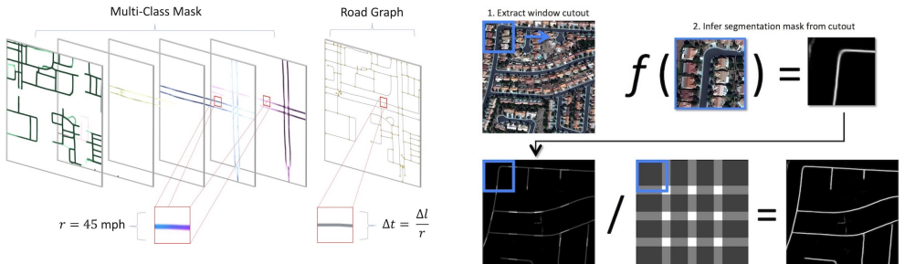
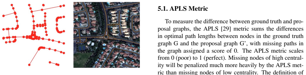
The central object is the multi-class road mask: a seven-channel per-pixel prediction whose channels bin road speeds into 1-10 mph through 61-70 mph ranges. This mask does double duty: it locates roads and labels their speed in one pass, and after skeletonization it supplies per-segment speed estimates via 8x8 pixel patches at segment midpoints. Those estimates become edge weights, so the graph supports the APLS metric (Average Path Length Similarity, a 0-to-1 graph-theoretic score comparing optimal path lengths in the proposal graph against the ground-truth graph) with travel time as the edge weight, turning a segmentation system into a routing system.
What would settle it
Collect observed travel times for one or more test cities from GPS probe traces or floating-car data, recompute APLS_time using those observed speeds as ground-truth edge weights instead of Table 7 speeds, and check whether the score still stays only about 4 percent below APLS_length; if it drops substantially, or if inferred speeds disagree systematically with observed speeds by road class, the claim that time-optimized routing is feasible from imagery alone would be refuted.
Extended reading notes
Core claim
The paper claims that a road graph extracted purely from satellite imagery can be weighted by estimated travel time, enabling true time-optimized routing rather than only shortest-geographic-distance routing. It demonstrates this by training a segmentation network on multi-channel masks whose channels correspond to 10 mph speed bins, skeletonizing the predicted mask into a graph, sampling 8x8 prediction patches at each segment midpoint to estimate speed, and computing edge travel time as length divided by speed. On large-area tests spanning four cities, the method scores APLS length = 0.67 and APLS time = 0.64, a 4 percent drop, which the paper interprets as evidence that travel-time labels are informative enough for routing. The paper also reports a 5 percent improvement over prior work on one benchmark and a 23 percent improvement over a prior baseline on another, while emphasizing that the speed inference itself is the new contribution.
Load-bearing premise
The travel-time result rests on the assumption that speeds synthesized from road metadata via Table 7 (road type, lane count, surface) are a valid proxy for actual travel times; the evaluation compares the model's predictions against those same synthesized labels, so the time-optimization claim is internally consistent rather than validated against observed traffic.
Editorial extensions
If this is right
- A satellite-imagery pipeline can supply a routable road graph with travel-time edge weights, so time-sensitive navigation need not wait for manual map updates.
- Because the APLS time score is only about 4 percent lower than APLS length on large test areas, routing by inferred travel time should be nearly as reliable as routing by geometry on the extracted graph.
- The pipeline runs at about 280 square kilometers per hour per GPU, so a small GPU cluster could produce a fresh road-and-time map of a disaster area in hours rather than the weeks a human mapping team needs.
- The multi-class speed mask couples road detection with speed labels, so road topology and travel-time metadata are extracted in a single pass rather than as separate stages.
- Complex intersections and dense urban interchanges remain failure points, so graphs extracted by this method will need gap-closing care before use in routing at complex junctions.
Reading between the lines
- The paper's time scores are computed against speed labels synthesized from road metadata, not measured traffic; a direct validation against GPS probe speeds would be the true test of whether time-optimized routing works in practice.
- The same pipeline could be re-run on fresh imagery of the same area to update speed estimates after disasters or road changes, since nothing in the method depends on a static map database.
- Because speed labels derive from road class rather than real congestion, the method recovers typical posted-speed orderings, not dynamic conditions; using it for real-time traffic routing would require a congestion signal or a model that learns temporal patterns.
- The continuous-mask variant's tendency to overestimate high-confidence speeds suggests that a calibration or regression head could yield smoother speed estimates than 10 mph bins, a natural next step for routed applications.
Signed reviews
Editorial analysis
A structured set of objections, weighed in public.
Referee Report
Summary. This paper presents CRESIv2, an extension of prior road-extraction work that adds prediction of road speed limits and travel times from satellite imagery. The method uses multi-class segmentation masks with speed bins, graph extraction via skeletonization, and assigns each edge a mean speed estimated from patches of the predicted mask. Experiments on SpaceNet and Google/OSM imagery report state-of-the-art APLS/TOPO scores for road extraction, and APLS time scores that the authors interpret as evidence that time-optimized routing is feasible.
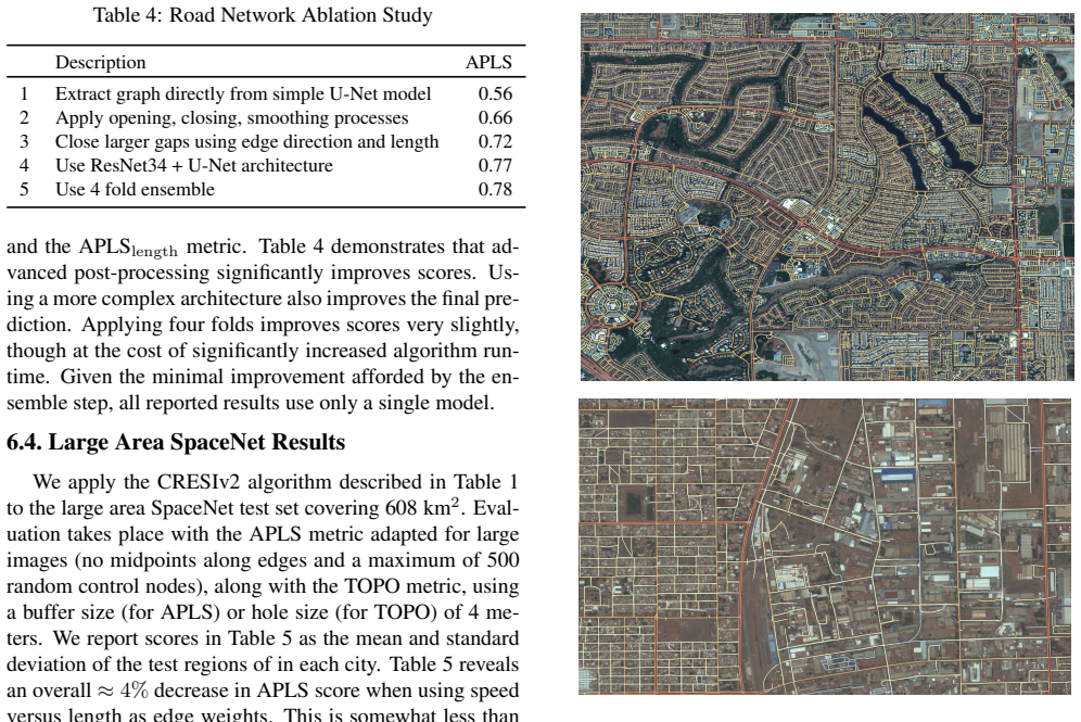
Significance. The road-extraction contribution is solid: an ablation study (Table 4), held-out city evaluation (Table 5), public code, and consistent improvements over previous methods give confidence in the graph-extraction results. However, the speed/travel-time contribution is not validated against any independent ground truth: the target speed labels are generated by the authors' own mapping (Table 7, Oregon guidelines) and applied uniformly to Paris, Shanghai, Khartoum, and Las Vegas. The APLS time metric measures agreement with these synthetic labels, so the paper's central claim—that estimated travel times permit true optimal routing—is not established by the evidence presented.
major comments (4)
- [Section 4 and Appendix A] The central claim requires external validation of the speed estimates. The ground-truth speeds are not measured data but are produced by the authors' Table 7 mapping from road metadata to speed, using Oregon guidelines for cities on three continents. The model is trained to predict these synthetic labels, and the APLS time metric in Section 6.4 evaluates against the same labels. Thus the reported APLS time scores demonstrate that the model can reproduce the authors' heuristic from imagery, not that the predicted speeds correspond to real-world travel times. This is a load-bearing limitation for the paper's main novelty. I recommend either validating the speed predictions against independent data (e.g., OSM maxspeed tags, GPS trajectories, or commercial routing APIs) or substantially reframing the claims to refer to 'metadata-derived speed estimates' rather than actual travel times.
- [Section 7] The statement 'The aggregate score of APLS time = 0.64 implies that travel time estimates will be within ≈ 1/3 of the ground truth' is not supported by the metric. APLS is a graph-level path-similarity measure, not a per-edge speed error bound. A graph-level score of 0.64 can be obtained with widely varying per-edge speed errors, and the relationship between APLS and per-edge error is not characterized. This sentence should be removed or replaced with a direct error analysis, such as per-edge speed MAE or median relative error.
- [Section 3.4] The multi-class speed estimation procedure is underspecified. The text says that 'if the majority of the high confidence pixels in the prediction mask patch belong to channel 3 ... we would assign the speed at that patch to be 35 mph,' but it does not define how the channel probabilities are combined, how 'majority' is determined, or how the final per-edge speed is computed when different patches yield different speeds. This level of detail is needed for reproducibility and for interpreting the APLS time results. Please specify the exact algorithm, including the handling of ties and low-confidence pixels.
- [Section 6.4 and Table 5] The conclusion that 'routing based on time shows only a 3–13% decrease' does not demonstrate that speed inference is accurate. Because all speeds are derived from a narrow range (10–65 mph) and the evaluation target is the authors' own Table 7 mapping, the small APLS length-to-time gap could simply reflect the compressed speed distribution. The paper would benefit from a direct routing experiment (e.g., comparing fastest-path versus shortest-path travel times using independent speed data) or at minimum a discussion of this confound. Without such evidence, the claim that 'true time-optimized routing is possible' remains unsupported.
minor comments (6)
- [Section 3.3] Typo: 'sckit-image' should be 'scikit-image'.
- [Figure 5 caption] Typo: 'arbitarily' should be 'arbitrarily'.
- [Section 6.3] Duplicate word: 'we utilize the the same subset' should read 'we utilize the same subset'.
- [Section 5.1 and Throughout] The metric names 'APLSlength' and 'APLS time' are formatted inconsistently; use a consistent notation such as 'APLS_length' and 'APLS_time' or spelled-out forms.
- [Appendix B, Table 8] The Khartoum 0 row appears to contain a formatting error: '0 3.0' likely should be '0.3'. Please correct the table.
- [Section 6.2] The 60–100% improvement claim in the text is not directly visible in Table 3; please clarify the exact computation (e.g., 0.77/0.39 - 1) so readers can reproduce the stated figure.
Circularity Check
Travel-time claim is validated only against internally defined Table 7 speeds; APLS time measures self-consistency with the authors' own heuristic rather than real-world routing.
-
self definitional
[Section 4 / Appendix A / Section 5.1 / Section 7]
"Speed is assigned with Table 7, using the Oregon guidelines for road speed [22]... if we assign a travel time estimate to each graph edge we can use the APLS time metric to measure differences in travel times between ground truth and proposal graphs... The aggregate score of APLS time = 0.64 implies that travel time estimates will be within≈ 1/3 of the ground truth."
The ground-truth travel times used in the APLStime benchmark are not measured travel times; they are computed from speeds assigned in Table 7 according to road metadata. The same metadata-derived speeds are used to construct the multi-class and continuous training masks (Section 3.1/3.2), so the model is trained to predict exactly the label that Table 7 defines. Evaluating APLStime against those same Table 7-derived labels therefore measures only how well the model reproduces the authors' own speed heuristic from imagery on held-out cities. The claim that 'travel time estimates will be within 1/3 of the ground truth' is thus relative to an internally constructed definition of ground truth, not to real-world travel times or independent speed observations.
full rationale
The only substantive circularity candidate is the travel-time evaluation. The paper assigns speed limits using Table 7, builds training masks from those assigned speeds, trains CRESIv2 to predict those masks, and then computes APLStime using the same Table 7-derived speeds as ground truth. Consequently APLStime = 0.64 shows that the model can recover the author-defined metadata-to-speed mapping from imagery on held-out cities; it does not validate the mapping against observed speed data or demonstrate that resulting routes are time-optimal. This is a real internal-consistency limitation, so I score it 4 rather than 0. It is not a pure tautology: the test cities are held out and the model must generalize the mapping from visual features, so the result has independent information content about how well the heuristic can be inferred from imagery. The geometric and topological results (APLSlength, TOPO) and the Google/OSM comparison are benchmarked against external labels and prior work, so they are not circular. Citations to the author's own CRESI v1 and SpaceNet papers provide data and prior implementation context, but no load-bearing derivation reduces to those self-citations; the central geometric extraction claims are self-contained against external benchmarks. The main weakness is external validity of the speed labels, not derivation circularity.
Assumptions & free parameters
free parameters (6)
- Road mask halfwidth =
2 m
- Speed mapping table (Table 7) =
10-65 mph by road type, lanes, surface; non-paved multiplied by 0.75
- Speed bin width =
10 mph bins (1-70 mph)
- Loss weight alpha_mc / alpha_c =
0.75
- Gap closing and pruning thresholds =
6 m/80 m minimum subgraph, 3 m terminal edge, 6 m connection distance
- Evaluation buffer/hole size =
4 m (and 15 m for TOPO comparison)
assumptions (4)
- domain assumption Road speed can be estimated from road type, number of lanes, and surface type.
- domain assumption Speed limit is constant along each road edge.
- domain assumption The APLS time metric, computed against metadata-derived speeds, reflects routing quality.
- standard math Skeletonization of the segmentation mask yields a graph faithful to the road network.
Cite this review
Pith. "Pith review of City-Scale Road Extraction from Satellite Imagery v2: Road Speeds and Travel Times." pith.science (2026). https://pith.science/paper/F4RAVTZO
@misc{pith2026190809715,
  author       = {Pith},
  title        = {Pith review of: City-Scale Road Extraction from Satellite Imagery v2: Road Speeds and Travel Times},
  year         = {2026},
  howpublished = {\url{https://pith.science/paper/F4RAVTZO}},
  note         = {Machine review of arXiv:1908.09715}
}
read the original abstract
Automated road network extraction from remote sensing imagery remains a significant challenge despite its importance in a broad array of applications. To this end, we explore road network extraction at scale with inference of semantic features of the graph, identifying speed limits and route travel times for each roadway. We call this approach City-Scale Road Extraction from Satellite Imagery v2 (CRESIv2), Including estimates for travel time permits true optimal routing (rather than just the shortest geographic distance), which is not possible with existing remote sensing imagery based methods. We evaluate our method using two sources of labels (OpenStreetMap, and those from the SpaceNet dataset), and find that models both trained and tested on SpaceNet labels outperform OpenStreetMap labels by greater than 60%. We quantify the performance of our algorithm with the Average Path Length Similarity (APLS) and map topology (TOPO) graph-theoretic metrics over a diverse test area covering four cities in the SpaceNet dataset. For a traditional edge weight of geometric distance, we find an aggregate of 5% improvement over existing methods for SpaceNet data. We also test our algorithm on Google satellite imagery with OpenStreetMap labels, and find a 23% improvement over previous work. Metric scores decrease by only 4% on large graphs when using travel time rather than geometric distance for edge weights, indicating that optimizing routing for travel time is feasible with this approach.
Figures


Figures from the paper (12 more)




Reference graph
Works this paper leans on
-
[1]
Spacenet round 3 winner: albu’s implementation
albu. Spacenet round 3 winner: albu’s implementation. https://github.com/SpaceNetChallenge/ RoadDetector/tree/master/albu-solution, 2018
work page 2018
-
[2]
F. Bastani. fbastani spacenet solution. https://github. com/SpaceNetChallenge/RoadDetector/tree/ master/fbastani-solution, 2018
work page 2018
-
[3]
F. Bastani, S. He, M. Alizadeh, H. Balakrishnan, S. Madden, S. Chawla, S. Abbar, and D. DeWitt. RoadTracer: Auto- matic Extraction of Road Networks from Aerial Images. In Computer Vision and Pattern Recognition (CVPR), Salt Lake City, UT, June 2018
work page 2018
- [4]
-
[5]
J. Biagioni and J. Eriksson. Inferring road maps from global positioning system traces: Survey and comparative evalua- tion. Transportation Research Record, 2291(1):61–71, 2012
work page 2012
-
[6]
D. Chai, W. Frstner, and F. Lafarge. Recovering line- networks in images by junction-point processes. In 2013 IEEE Conference on Computer Vision and Pattern Recog- nition, pages 1894–1901, June 2013
work page 2013
-
[7]
Broad area satellite imagery semantic seg- mentation
CosmiQWorks. Broad area satellite imagery semantic seg- mentation. https://github.com/CosmiQ/basiss, 2018
work page 2018
-
[8]
M. CSAIL. Roadtracer: Automatic extraction of road networks from aerial images. https://roadmaps. csail.mit.edu/roadtracer/, 2018
work page 2018
Show all 35 references
-
[9]
Demir, K
I. Demir, K. Koperski, D. Lindenbaum, G. Pang, J. Huang, S. Basu, F. Hughes, D. Tuia, and R. Raska. Deepglobe 2018: A challenge to parse the earth through satellite images. In 2018 IEEE/CVF Conference on Computer Vision and Pat- tern Recognition Workshops (CVPRW) , pages 172–1...
2018
-
[10]
A. V . Etten. City-scale road extraction from satellite imagery. CoRR, abs/1904.09901, 2019
1904 arXiv
-
[11]
A. A. Hagberg, D. A. Schult, and P. J. Swart. Exploring net- work structure, dynamics, and function using networkx. In G. Varoquaux, T. Vaught, and J. Millman, editors, Proceed- ings of the 7th Python in Science Conference, pages 11 – 15, Pasadena, CA USA, 2008
2008
-
[12]
K. He, X. Zhang, S. Ren, and J. Sun. Deep residual learning for image recognition. In 2016 IEEE Conference on Com- puter Vision and Pattern Recognition (CVPR) , pages 770– 778, June 2016
2016
-
[13]
2d semantic labeling contest
ISPRS. 2d semantic labeling contest. http: //www2.isprs.org/commissions/comm3/wg4/ semantic-labeling.html, 2018
2018
-
[14]
T. Lin, P. Goyal, R. Girshick, K. He, and P. Dollar. Focal loss for dense object detection. IEEE Transactions on Pattern Analysis and Machine Intelligence, pages 1–1, 2018
2018
-
[15]
V . Mnih. Machine Learning for Aerial Image Labeling. PhD thesis, University of Toronto, 2013
2013
-
[16]
Mnih and G
V . Mnih and G. E. Hinton. Learning to detect roads in high- resolution aerial images. In K. Daniilidis, P. Maragos, and N. Paragios, editors, Computer Vision – ECCV 2010 , pages 210–223, Berlin, Heidelberg, 2010. Springer Berlin Heidel- berg
2010
-
[17]
Mosinska, P
A. Mosinska, P. M ´arquez-Neila, M. Kozinski, and P. Fua. Beyond the pixel-wise loss for topology-aware delineation. 2018 IEEE/CVF Conference on Computer Vision and Pat- tern Recognition, pages 3136–3145, 2017
2018
-
[18]
Mttyus, W
G. Mttyus, W. Luo, and R. Urtasun. Deeproadmapper: Ex- tracting road topology from aerial images. In 2017 IEEE International Conference on Computer Vision (ICCV), pages 3458–3466, Oct 2017
2017
-
[19]
Mttyus, S
G. Mttyus, S. Wang, S. Fidler, and R. Urtasun. Enhanc- ing road maps by parsing aerial images around the world. In 2015 IEEE International Conference on Computer Vision (ICCV), pages 1689–1697, Dec 2015
2015
-
[20]
Mttyus, S
G. Mttyus, S. Wang, S. Fidler, and R. Urtasun. Hd maps: Fine-grained road segmentation by parsing ground and aerial images. In 2016 IEEE Conference on Computer Vision and Pattern Recognition (CVPR), pages 3611–3619, June 2016
2016
-
[21]
2017 hurricanes irma and maria
OpenStreetMap. 2017 hurricanes irma and maria. https://wiki.openstreetmap.org/wiki/ 2017_Hurricanes_Irma_and_Maria, 2017
2017
-
[22]
Osm tags for routing/maxspeed
OpenStreetMap. Osm tags for routing/maxspeed. https://wiki.openstreetmap.org/wiki/ OSM_tags_for_routing/Maxspeed#United_ States_of_America, 01 2019
2019
-
[23]
Planet dump re- trieved from https://planet.osm.org
OpenStreetMap contributors. Planet dump re- trieved from https://planet.osm.org . https: //www.openstreetmap.org, 2019
2019
-
[24]
Ronneberger, P
O. Ronneberger, P. Fischer, and T. Brox. U-net: Convo- lutional networks for biomedical image segmentation. In N. Navab, J. Hornegger, W. M. Wells, and A. F. Frangi, editors, Medical Image Computing and Computer-Assisted Intervention – MICCAI 2015 , pages 234–241, Cham, 2015. ...
2015
-
[25]
Skeletonize
scikit image. Skeletonize. https://scikit-image. org/docs/dev/auto_examples/edges/plot_ skeleton.html, 2018
2018
-
[26]
Sironi, V
A. Sironi, V . Lepetit, and P. Fua. Multiscale centerline de- tection by learning a scale-space distance transform. In 2014 IEEE Conference on Computer Vision and Pattern Recogni- tion, pages 2697–2704, June 2014
2014
-
[27]
Stoica, X
R. Stoica, X. Descombes, and J. Zerubia. A gibbs point pro- cess for road extraction from remotely sensed images. Inter- national Journal of Computer Vision, 57:121–136, 05 2004
2004
-
[28]
Tretken, F
E. Tretken, F. Benmansour, B. Andres, H. Pfister, and P. Fua. Reconstructing loopy curvilinear structures using integer programming. In 2013 IEEE Conference on Computer Vi- sion and Pattern Recognition, pages 1822–1829, June 2013
2013
-
[29]
Van Etten, D
A. Van Etten, D. Lindenbaum, and T. M. Bacastow. SpaceNet: A Remote Sensing Dataset and Challenge Series. ArXiv e-prints, July 2018
2018
-
[30]
J. Wang, Q. Qin, Z. Gao, J. Zhao, and X. Ye. A new approach to urban road extraction using high-resolution aerial image. ISPRS International Journal of Geo-Information, 5(7), 2016
2016
-
[31]
S. Wang, M. Bai, G. M ´attyus, H. Chu, W. Luo, B. Yang, J. Liang, J. Cheverie, S. Fidler, and R. Urtasun. Toron- tocity: Seeing the world with a million eyes. CoRR, abs/1612.00423, 2016
2016 arXiv
-
[32]
J. D. Wegner, J. A. Montoya-Zegarra, and K. Schindler. A higher-order crf model for road network extraction. In 2013 IEEE Conference on Computer Vision and Pattern Recogni- tion, pages 1698–1705, June 2013
2013
-
[33]
Skeleton network
yxdragon. Skeleton network. https://github.com/ yxdragon/sknw, 2018
2018
-
[34]
Zhang, Q
Z. Zhang, Q. Liu, and Y . Wang. Road extraction by deep residual u-net. IEEE Geoscience and Remote Sensing Let- ters, 15:749–753, 2018
2018
-
[35]
L. Zhou, C. Zhang, and M. Wu. D-linknet: Linknet with pretrained encoder and dilated convolution for high resolu- tion satellite imagery road extraction. pages 192–1924, 06 2018. Appendix A. Road Speed Assignment See [29] for details on the precise labeling guidelines and road...
1924
Reviewed August 14, 2026 · model on record in the stance chip above.
Discussion (0). Continue with ORCID to comment.