REVIEW 4 major objections 6 minor 34 references
EFKAN: A KAN-Integrated Neural Operator For Efficient Magnetotelluric Forward Modeling
T0 review · 4 major / 6 minor · reviewed 2026-08-09 · deepseek-v4-flash
Pith's one-line read EFKAN predicts magnetotelluric apparent resistivity and phase more accurately than the MLP-based EFNO, while running about 1000 times faster than finite-difference forward modeling.
desk verdict A KAN-for-MLP swap in EFNO for 2D MT forward modeling; the speedup is real, but the accuracy claim over EFNO fails on the paper's own generalization tests. read the letter →
The pith
A machine-rendered reading of the paper's core claim, the machinery that carries it, and where it could break.
The reading
What carries the argument
The load-bearing object is the EFKAN architecture itself: the DeepONet decomposition $G(\sigma)(y,z,f) \approx \sum_k b_k(\sigma)\, t_k(y,z,f)$, with $b_k$ computed by an FNO branch (six Fourier layers, $k_{\max}=18$, GELU activations) and $t_k$ by a KAN trunk (three layers, widths 2–256–4096, grid size 5, spline order 3). KAN replaces each linear weight by a learnable univariate function, here a weighted sum of a basis function and a B-spline; the paper credits this locality and adjustability for the improved accuracy and training stability. The synthetic training distribution is produced with the spectral method using power spectrum $P(k)\propto |k|^{-\beta/2}$ for $\beta\in\{3,\ldots,7\}$, aimed at mimicking smooth geological conductivity variations.
What would settle it
Average the relative $\ell^1$ errors over all 100 samples of testing dataset B: Table 4 already shows EFKAN at 0.0884 versus EFNO at 0.0819, so if that reversal is representative, the claim that EFKAN is more accurate than EFNO fails for the unseen-anomaly case.
Extended reading notes
Core claim
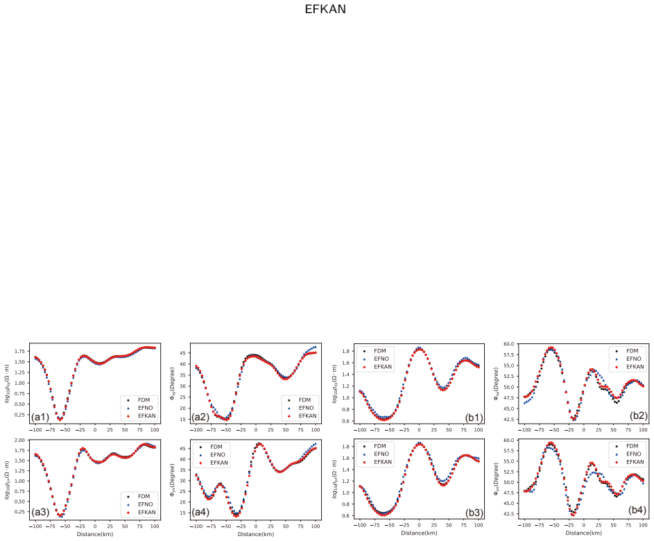
EFKAN is a DeepONet-style operator in which a six-layer Fourier neural operator serves as the branch, encoding the 2-D resistivity model $\rho(y,z)$, and a three-layer Kolmogorov-Arnold network serves as the trunk, encoding the queried surface coordinates and frequencies $(y,z,f)$; the apparent resistivities $\rho_{xy},\rho_{yx}$ and phases $\phi_{xy},\phi_{yx}$ are recovered as the branch–trunk inner product. The paper's central claim is that this KAN-for-MLP swap improves accuracy: EFKAN reports lower mean relative $\ell^1$ error than EFNO on in-distribution test set A and on entirely unseen frequencies (test set C), and better fits to the finite-difference ground truth on rectangular-anomaly models, while taking about 0.01 seconds per model versus about 10 seconds for FDM. The paper also reports smoother convergence and retention of accuracy when training is downsampled to 22 frequencies/coordinates or downscaled to 5,000 samples.
Load-bearing premise
All accuracy claims rest on the assumption that the synthetic training distribution—smooth Gaussian random fields with spectral exponents $\beta=3$–7, plus rectangular anomalies in testing—is representative enough of real subsurface conductivity structures for the reported gains to carry over to field data.
Editorial extensions
If this is right
- An MT inversion could afford orders of magnitude more forward solves per iteration, making global or stochastic searches feasible at a fraction of the current cost.
- Because EFKAN outputs responses at arbitrary query points and frequencies, inversions can be evaluated exactly at the field stations and periods of an observed dataset without retraining the surrogate.
- The reported accuracy from training on 22 frequencies/coordinates or on 5,000 samples suggests the surrogate can be deployed in data-scarce geoscience settings with modest synthetic training sets.
- The smoother loss curves and lower final loss than EFNO indicate that KAN trunks are a viable drop-in replacement for MLP trunks in operator learning for PDEs.
Reading between the lines
- Because B-spline KANs are not GPU-parallelized, EFKAN is slower per query than EFNO (roughly 1.1 s vs 0.2 s per 100 models in the paper's tables); testing the paper's suggested alternatives—radial basis functions, wavelets, or Jacobi polynomials—would show whether the accuracy gain can be combined with EFNO-level speed.
- The accuracy gain may come from the trunk's learnable univariate functions rather than from KAN as such; an ablation comparing EFKAN with another learnable-activation trunk at matched parameter count and training budget would isolate the mechanism.
- The training distribution is smooth Gaussian random fields, so the decisive out-of-distribution test is real-world structures with sharp faults, salt flanks, or thin layers; evaluating on such models or on field MT data would show whether the reported accuracy survives where it matters.
- The same FNO-branch/KAN-trunk split should transfer to 3-D MT forward modeling, but the paper demonstrates only 2-D; a 3-D extension is the natural next step to test before use in 3-D inversion.
Editorial analysis
A structured set of objections, weighed in public.
Referee Report
Summary. The paper proposes EFKAN, a neural operator for 2D magnetotelluric forward modeling that combines a Fourier neural operator (FNO) as the branch network with a Kolmogorov-Arnold network (KAN) as the trunk network. The trunk maps the branch output to apparent resistivity and phase at arbitrary receiver locations and frequencies. The method is trained on synthetic resistivity models generated with the spectral method (Gaussian random fields, beta 3-7) plus rectangular anomaly test cases, and is compared against EFNO, an FNO-with-MLP-trunk baseline, with finite-difference method (FDM) solutions as ground truth. The paper claims higher accuracy than EFNO and roughly 1000x speedup over FDM, and reports experiments on the original training dataset, a downsampled frequency/coordinate dataset, and a reduced-sample dataset.
Significance. If the accuracy claims held across all test distributions, EFKAN would be a useful surrogate for rapid 2D MT forward modeling, with the practical advantage of evaluating responses at arbitrary locations and frequencies. The paper has clear strengths: predictions are benchmarked against FDM solutions (an external reference, so the evaluation is not circular), the source code is publicly available, and the experimental design includes several meaningful generalization tests (unseen rectangular anomalies, unseen frequencies, downsampled training data, and reduced training data). The central weakness is that the unqualified accuracy advantage over EFNO is not supported by the paper's own aggregate and per-component results on the out-of-distribution tests, and the baseline comparison is not controlled for model capacity or optimization variance.
major comments (4)
- [Table 4 and Discussion] The Discussion states without qualification that EFKAN 'can achieve higher accuracy in apparent resistivity and phase measurements compared to the EFNO,' but Table 4 contradicts this on the out-of-distribution tests: on testing dataset B, EFKAN has larger average l1 error than EFNO (0.0884 vs 0.0819), and on dataset C the two are essentially tied (0.0776 vs 0.0785). The per-component errors reported in Section 3.2 also favor EFNO for several quantities on datasets B and C, for example rho_xy 0.0908 vs 0.0826 and rho_yx 0.0969 vs 0.0867 on B, and rho_xy 0.0451 vs 0.0391 and phi_yx 0.1485 vs 0.1349 on C. The accuracy claim needs to be re-scoped to the same-distribution setting, and the paper should discuss why the in-domain gain does not transfer to the generalization tests that are most relevant for field deployment.
- [Section 2.2.3 and Tables 1-2] The EFNO baseline is uncontrolled: the MLP trunk architecture, layer widths, and parameter count of EFNO are never reported, while the KAN trunk used in EFKAN has 4096 hidden neurons in its final layer (Table 2). The same-distribution accuracy gain on testing dataset A could therefore reflect larger model capacity or different optimization behavior rather than a KAN-specific advantage. A fair comparison should match the trunk capacity or explicitly report parameter counts for both models and demonstrate that the gain survives similar-capacity settings.
- [Section 3.2 and Tables 4-6] All accuracy comparisons are based on single runs: no repeated seeds, no standard deviations, and no statistical significance testing. Given that the aggregate differences on dataset C are tiny (0.0776 vs 0.0785), and that the per-component errors on datasets B and C frequently favor EFNO, the claim of higher accuracy requires at least a few random restarts and reporting of the resulting error distributions before it can be considered established.
- [Section 4] The Discussion claims that KAN endows EFKAN with 'a certain degree of interpretability' and that KAN reduces overfitting, but neither is demonstrated in the experiments. No learned spline functions are analyzed, and the generalization results on dataset B (where EFKAN is worse than EFNO) do not support an overfitting-reduction claim. These interpretive claims should either be supported with specific evidence or removed.
minor comments (6)
- [Section 3] The note that color bars differ between the EFNO and EFKAN error plots makes visual comparisons unreliable; the paper should use a common color scale or state explicitly that visual differences are not directly comparable.
- [Table 1 and Section 3.2] There are typos in the manuscript: 'bacth size' in Table 1, 'the the original training dataset dataset' in Section 3.2 and in figure captions, and 'ENKAN' in the Discussion.
- [Figure 15 caption] The caption reads 'The 1-D profiles in from Fig. 14' and should be corrected.
- [Section 4] The explanation for testing loss being lower than training loss is not convincing: Eq. (17) defines an average per-sample loss, so the larger number of training samples does not explain a higher average training loss. The authors should compare loss on a matched-size random subset of the training set or revise the explanation.
- [Data availability] The data availability statement says 'No data was used for the research described in the article,' but the study generates and uses synthetic datasets; this should be clarified to avoid confusion about whether the generated data are shared.
- [Abstract and Conclusion] The abstract and conclusion should carry the same qualification as the revised Discussion, namely that the accuracy advantage over EFNO is demonstrated on same-distribution data but not consistently on unseen rectangular anomalies and unseen frequencies.
Circularity Check
No circularity: EFKAN's predictions are trained and scored against independent FDM solutions; the disputed accuracy claims stem from uncontrolled baseline comparisons and conflicting Table 4 numbers, not from a self-referential derivation.
full rationale
The paper's core pipeline is a supervised surrogate-model evaluation: synthetic resistivity models are generated by a spectral/GRF method, labeled electromagnetic responses are produced by an external finite-difference solver, and both EFNO and EFKAN are trained to minimize a relative L1 loss against those FDM labels. The reported test errors on datasets A, B, and C are measured against the same external FDM ground truth, so the target quantities are not constructed from the model outputs or from fitted constants that are later renamed as predictions. The Kolmogorov-Arnold representation theorem and the KAN architecture are adopted from independent literature (Liu et al., 2024), and no uniqueness or forcing theorem from the present authors is invoked to justify the architecture. The only self-citation that appears in a load-bearing-looking sentence is the remark that test loss below training loss 'has also occurred in our previous work (Peng et al., 2022)', but that is anecdotal context and not an argument that establishes the paper's central accuracy claim. The legitimate concerns raised by the manuscript's own numbers — EFKAN is worse than EFNO on testing dataset B (0.0884 vs 0.0819) and essentially tied on dataset C (0.0776 vs 0.0785) in Table 4, while the MLP trunk of the EFNO baseline is never specified — are threats to the validity of the comparative accuracy claim, but they are experimental-design and internal-consistency issues, not circular derivations. No equation in the paper reduces to its inputs, no fitted parameter is relabeled as a prediction, and no self-citation chain carries the logical weight of the conclusion. Therefore, the appropriate finding is no significant circularity.
Assumptions & free parameters
free parameters (4)
- Fourier mode truncation kmax =
18
- KAN architecture hyperparameters =
3 layers, widths 2/256/4096, grid 5, spline order 3
- Spectral method beta values =
3, 4, 5, 6, 7
- Conductivity range and boundary values =
1e-4 to 1 S/m; air 1e-9; lower boundary 1e-2
assumptions (5)
- standard math Kolmogorov-Arnold representation theorem holds and is a useful basis for the trunk network.
- domain assumption Quasi-stationary field assumption and neglect of displacement current are valid for the MT frequency range.
- domain assumption The 2D MT problem decouples into xy and yx modes with Dirichlet boundary conditions.
- domain assumption FDM solutions at the chosen 64x64 grid are accurate enough to serve as ground truth.
- domain assumption GRF-generated synthetic resistivity models are representative of real MT targets.
Cite this review
Pith. "Pith review of EFKAN: A KAN-Integrated Neural Operator For Efficient Magnetotelluric Forward Modeling." pith.science (2026). https://pith.science/paper/FAKI3CNJ
@misc{pith2026250202195,
  author       = {Pith},
  title        = {Pith review of: EFKAN: A KAN-Integrated Neural Operator For Efficient Magnetotelluric Forward Modeling},
  year         = {2026},
  howpublished = {\url{https://pith.science/paper/FAKI3CNJ}},
  note         = {Machine review of arXiv:2502.02195}
}
read the original abstract
Magnetotelluric (MT) forward modeling is fundamental for improving the accuracy and efficiency of MT inversion. Neural operators (NOs) have been effectively used for rapid MT forward modeling, demonstrating their promising performance in solving the MT forward modeling-related partial differential equations (PDEs). Particularly, they can obtain the electromagnetic field at arbitrary locations and frequencies. In these NOs, the projection layers have been dominated by multi-layer perceptrons (MLPs), which may potentially reduce the accuracy of solution due to they usually suffer from the disadvantages of MLPs, such as lack of interpretability, overfitting, and so on. Therefore, to improve the accuracy of MT forward modeling with NOs and explore the potential alternatives to MLPs, we propose a novel neural operator by extending the Fourier neural operator (FNO) with Kolmogorov-Arnold network (EFKAN). Within the EFKAN framework, the FNO serves as the branch network to calculate the apparent resistivity and phase from the resistivity model in the frequency domain. Meanwhile, the KAN acts as the trunk network to project the resistivity and phase, determined by the FNO, to the desired locations and frequencies. Experimental results demonstrate that the proposed method not only achieves higher accuracy in obtaining apparent resistivity and phase compared to the NO equipped with MLPs at the desired frequencies and locations but also outperforms traditional numerical methods in terms of computational speed.
Figures


Figures from the paper (24 more)




Reference graph
Works this paper leans on
-
[1]
DeepOKAN:DeepOperatorNetworkBasedonKolmogorovArnoldNetworksforMechanics Problems
Abueidda,D.W.,Pantidis,P.,Mobasher,M.E.,2024. DeepOKAN:DeepOperatorNetworkBasedonKolmogorovArnoldNetworksforMechanics Problems. URL: http://arxiv.org/abs/2405.19143, doi:10.48550/arXiv.2405.19143. arXiv:2405.19143 [cs]. Bozdağ, E., Peter, D., Lefebvre, M., Komatitsch, D., Tromp, J., Hill, J., Podhorszki, N., Pugmire, D., . Global adjoint tomography: first...
-
[7]
Fluid transport and storage in the Cascadia forearc influenced by overriding plate lithology. Nature Geoscience 15, 677–682. URL:https://www.nature.com/articles/ s41561-022-00981-8, doi:10.1038/s41561-022-00981-8. Gao, J., Zhang, H., Zhang, S., Chen, X., Cheng, Z., Jia, X., Li, S., Fu, L., Gao, L., Xin, H.,
-
[10]
Geophysical Journal International 229, 1628–1645
Application of multiscale magnetotelluric data to mineral exploration: an example from the east Tennant region, Northern Australia. Geophysical Journal International 229, 1628–1645. URL: https://doi.org/10.1093/gji/ggac029, doi:10.1093/gji/ggac029. Kolmogorov, A.K.,
-
[12]
URL:http://arxiv.org/abs/2108.08481, doi:10.5555/3648699.3648788
Neural Operator: Learning Maps Between Function Spaces. URL:http://arxiv.org/abs/2108.08481, doi:10.5555/3648699.3648788. arXiv:2108.08481 [cs, math]. Li, Z.,
-
[13]
URL: http://arxiv.org/abs/2405.06721
Kolmogorov-Arnold Networks are Radial Basis Function Networks. URL: http://arxiv.org/abs/2405.06721. arXiv:2405.06721 [cs]. Li, Z., Kovachki, N., Azizzadenesheli, K., Liu, B., Bhattacharya, K., Stuart, A., Anandkumar, A.,
-
[14]
URL:http://arxiv.org/abs/2003.03485
Neural Operator: Graph Kernel Network for Partial Differential Equations. URL:http://arxiv.org/abs/2003.03485. arXiv:2003.03485 [cs, math, stat]. Li, Z., Kovachki, N., Azizzadenesheli, K., Liu, B., Bhattacharya, K., Stuart, A., Anandkumar, A.,
arXiv 2003
-
[16]
Swin Transformer: Hierarchical Vision Transformer using Shifted Windows, in: 2021 IEEE/CVF International Conference on Computer Vision (ICCV), IEEE, Montreal, QC, Canada. pp. 9992–10002. URL: https://ieeexplore.ieee.org/document/9710580/, doi:10.1109/ICCV48922.2021.00986. Liu, Z., Wang, Y., Vaidya, S., Ruehle, F., Halverson, J., Soljačić, M., Hou, T.Y., T...
-
[17]
URL: https://arxiv.org/abs/2404.19756v4
KAN: Kolmogorov-Arnold Networks. URL: https://arxiv.org/abs/2404.19756v4. Lu, L., Jin, P., Pang, G., Zhang, Z., Karniadakis, G.E.,
Show all 34 references
-
[18]
Nature Machine Intelligence 3, 218–229
Learning nonlinear operators via DeepONet based on the universal approximation theorem of operators. Nature Machine Intelligence 3, 218–229. URL: https://www.nature.com/articles/s42256-021-00302-5, doi:10.1038/s42256-021-00302-5. publisher: Nature Publishing Group. Newman, G.A...
-
[20]
Computers & Geosciences 176, 105360
Rapid surrogate modeling of magnetotelluric in the frequency domain using physics-driven deep neural networks. Computers & Geosciences 176, 105360. URL:https://linkinghub.elsevier.com/retrieve/pii/S009830042300064X, doi:10.1016/j.cageo.2023.105360. Peng, Z., Yang, B., Xu, Y., ...
-
[21]
IEEE Transactions on Geoscience and Remote Sensing 60, 1–12
Rapid Surrogate Modeling of Electromagnetic Data in Frequency Domain Using Neural Operator. IEEE Transactions on Geoscience and Remote Sensing 60, 1–12. doi:10.1109/TGRS.2022.3222507. conference Name: IEEE Transactions on Geoscience and Remote Sensing. Raissi, M., Perdikaris, ...
2022
-
[22]
Journal of Computational Physics 378, 686–707
Physics-informed neural networks: A deep learning framework for solving forward and inverse problems involving nonlinear partial differential equations. Journal of Computational Physics 378, 686–707. URL:https://www. sciencedirect.com/science/article/pii/S0021999118307125, doi...
-
[24]
IEEE Transactions on Geoscience and Remote Sensing 60, 1–9
Application of Multitask Learning for 2-D Modeling of Magnetotelluric Surveys: TE Case. IEEE Transactions on Geoscience and Remote Sensing 60, 1–9. URL:https://ieeexplore.ieee.org/document/9513472/, doi:10.1109/TGRS.2021.3101119. F. Wang, H. Qiu, Y. Huang, X. Gu, R. Wang, and ...
2021
-
[25]
URL:http://arxiv.org/abs/2406.02917
A comprehensive and FAIR comparison between MLP and KAN representations for differential equations and operator networks. URL:http://arxiv.org/abs/2406.02917. arXiv:2406.02917 [physics]. Siripunvaraporn, W., Egbert, G.,
-
[26]
Physics of theEarthandPlanetaryInteriors173,317–329
WSINV3DMT: Vertical magnetic field transfer function inversion and parallel implementation. Physics of theEarthandPlanetaryInteriors173,317–329. URL: https://www.sciencedirect.com/science/article/pii/S0031920109000144, doi:10.1016/j.pepi.2009.01.013. Smith, R.,
-
[27]
Electromagnetic Induction Methods in Mining Geophysics from 2008 to
2008
-
[30]
GEOPHYSICS 83, WB51–WB60
3D magnetotelluric modeling by using finite-difference method: Comparison study of different forward modeling approaches. GEOPHYSICS 83, WB51–WB60. URL: https://library.seg.org/doi/abs/10.1190/geo2017-0406.1, doi:10.1190/geo2017-0406.1. publisher: Society of Exploration Geophy...
-
[31]
JournalofGeophysicalResearch:SolidEarth125,e2020JB019396
New Insights Into Crustal and Mantle Flow Beneath the Red River Fault Zone and Adjacent Areas on the Southern Margin of the Tibetan Plateau Revealed by a 3-D Magnetotelluric Study. JournalofGeophysicalResearch:SolidEarth125,e2020JB019396. URL: https://agupubs.onlinelibrary.wil...
-
[33]
A Maxwell’s Equations Based Deep Learning Method for Time Domain Electromagnetic Simulations, in: 2020 IEEE Texas Symposium on Wireless and Microwave Circuits and Systems (WMCS), pp. 1–4. URL: https://ieeexplore.ieee.org/document/9172407, doi:10.1109/WMCS49442.2020.9172407. Zh...
2020
-
[34]
IEEE Transactions on Geoscience and Remote Sensing 60, 1–14
A Scalable Parallel Algorithm for 3-D Magnetotelluric Finite Element Modeling in Anisotropic Media. IEEE Transactions on Geoscience and Remote Sensing 60, 1–14. URL:https://ieeexplore.ieee.org/document/9438942/, doi:10.1109/TGRS.2021.3078735. F. Wang, H. Qiu, Y. Huang, X. Gu, ...
-
[1957]
Doklady Akademii Nauk SSSR 114, 369–373
On the Representation of Continuous Functions of Several Variables by Superposition of Continuous Functions of One Variable and Addition. Doklady Akademii Nauk SSSR 114, 369–373. F. Wang, H. Qiu, Y. Huang, X. Gu, R. Wang, and B. Yang:Preprint submitted to Elsevier Page 18 of 2...
2024
-
[1995]
IEEE Transactions on Neural Networks 6, 911–917
Universal approximation to nonlinear operators by neural networks with arbitrary activation functions and its application to dynamical systems. IEEE Transactions on Neural Networks 6, 911–917. URL:http://ieeexplore.ieee.org/document/ 392253/, doi:10.1109/72.392253. Varilsuha, ...
-
[2000]
Geophysical Journal International 140, 410–424
Three-dimensional magnetotelluric inversion using non-linear conjugate gradients. Geophysical Journal International 140, 410–424. URL: https://doi.org/10.1046/j.1365-246x.2000.00007.x, doi:10.1046/j.1365-246x. 2000.00007.x. Peng, Z., Yang, B., Liu, L., Xu, Y.,
-
[2009]
Constructive Approximation 30, 653–675
On a Constructive Proof of Kolmogorov’s Superposition Theorem. Constructive Approximation 30, 653–675. URL: https://doi.org/10.1007/s00365-009-9054-2, doi:10.1007/s00365-009-9054-2. Cheng, Y., Pang, Z., Kong, Y., Chen, X., Wang, G.,
-
[2012]
URL: http://link.springer.com/10.1007/s10712-013-9227-1, doi:10.1007/s10712-013-9227-1
Surveys in Geophysics 35, 123–156. URL: http://link.springer.com/10.1007/s10712-013-9227-1, doi:10.1007/s10712-013-9227-1. SS,S.,AR,K.,R,G.,KP,A.,2024. ChebyshevPolynomial-BasedKolmogorov-ArnoldNetworks:AnEfficientArchitectureforNonlinearFunction Approximation. URL:http://arxi...
2024 arXiv
-
[2014]
Geophysical Journal International 197, 1425–1441
On the sensitivity of long-term magnetotelluric monitoring in Southern Italy and source-dependent robust single station transfer function variability. Geophysical Journal International 197, 1425–1441. URL: https://doi.org/10.1093/gji/ggu083, doi:10.1093/gji/ggu083. Shan, T., G...
-
[2018]
Geothermics76,15–25
Three-dimensional magnetotelluric imaging of thegeothermalsystembeneaththeGongheBasin,NortheastTibetanPlateau. Geothermics76,15–25. URL: https://www.sciencedirect. com/science/article/pii/S0375650518300245, doi:10.1016/j.geothermics.2018.06.009. Guo, Z., Egbert, G., Dong, H., Wei, W.,
-
[2019]
Computers & Geosciences 127, 44–52
Inverting magnetotelluric responses in a three-dimensional earth using fast forward approximations based on artificial neural networks. Computers & Geosciences 127, 44–52. URL:https://www.sciencedirect. com/science/article/pii/S009830041830462X, doi:10.1016/j.cageo.2019.03.002...
-
[2020]
PhysicsoftheEarthandPlanetaryInteriors309,106585
Modular finite volume approach for 3D magnetotelluric modeling of the Earth medium with generalanisotropy. PhysicsoftheEarthandPlanetaryInteriors309,106585. URL: https://linkinghub.elsevier.com/retrieve/pii/ S0031920120302260, doi:10.1016/j.pepi.2020.106585. Jiang, W., Duan, J...
-
[2021]
URL:http://arxiv.org/abs/2010.08895
Fourier Neural Operator for Parametric Partial Differential Equations. URL:http://arxiv.org/abs/2010.08895. arXiv:2010.08895 [cs, math]. Liu, Z., Lin, Y., Cao, Y., Hu, H., Wei, Y., Zhang, Z., Lin, S., Guo, B.,
2010 arXiv
-
[2022]
Geothermics102,102386
Imaging the heat source of the Kangding high-temperature geothermal system on the Xianshuihefaultbymagnetotelluricsurvey. Geothermics102,102386. URL: https://www.sciencedirect.com/science/article/pii/ S0375650522000384, doi:10.1016/j.geothermics.2022.102386. Conway, D., Alexan...
-
[2023]
URL:http://arxiv.org/abs/2305
Interpretable Machine Learning for Science with PySR and SymbolicRegression.jl. URL:http://arxiv.org/abs/2305. 01582. arXiv:2305.01582 [astro-ph, physics:physics]. Egbert, G.D., Yang, B., Bedrosian, P.A., Key, K., Livelybrooks, D.W., Schultz, A., Kelbert, A., Parris, B.,
-
[2024]
URL: http://arxiv.org/abs/2405.12832
Wav-KAN: Wavelet Kolmogorov-Arnold Networks. URL: http://arxiv.org/abs/2405.12832. arXiv:2405.12832 [cs, eess, stat]. Braun, J., Griebel, M.,
-
[2025]
Computers & Geosciences 194, 105765
A two-dimensional magnetotelluric deep learning inversion approach based on improved Dense Convolutional Network. Computers & Geosciences 194, 105765. URL: https://www.sciencedirect.com/science/article/pii/ S0098300424002486, doi:10.1016/j.cageo.2024.105765. Yu, N., Zhang, H.,...
Reviewed August 9, 2026 · model on record in the stance chip above.
Discussion (0). Continue with ORCID to comment.