REVIEW 4 major objections 6 minor 51 references
Spatially-Enhanced Temporal Fusion Transformer: Interpretable Multi-Output Prediction for Parametric Dynamical Systems with Time-Varying Inputs
T0 review · 4 major / 6 minor · reviewed 2026-08-16 · deepseek-v4-flash
Pith's one-line read The paper claims that a transformer with block-wise masked attention can predict all future outputs of a parametric dynamical system in a single pass from the initial output, parameters, and known future input signal.
desk verdict A clean, small extension of TFT to multi-output surrogates with a nice attention-mask idea, but the evidence base is too narrow and the abstract overclaims. read the letter →
The pith
A machine-rendered reading of the paper's core claim, the machinery that carries it, and where it could break.
The reading
What carries the argument
The load-bearing object is the block-wise masked interpretable multi-head attention weight matrix $\tilde{A} \in \mathbb{R}^{(n_o n_t)\times(n_o n_t)}$, obtained after the data reshaping of Eq. (3) merges the output dimension into the temporal dimension. The causal mask is applied block-by-block instead of entry-by-entry: the block for time $t_i$ and $t_j$ with $i<j$ is masked, while every pair inside an unmasked block remains visible, so the model learns output-to-output interactions at each time step. The matrix therefore carries the temporal correlations of the original TFT and adds the spatial correlations between outputs, which is the mechanism that makes multi-output prediction interpretable in a single pass. The proof of Theorem 3.1 supplies the loss foundation: the quantile loss of TFT at $q=0.5$ equals half the MAE loss, so the MAE point forecasts used here are exactly the original TFT objective up to scaling.
What would settle it
Take a two-state oscillator with state $(x, v)$ and output $y = x$; generate two trajectories with the same parameters and the same initial output $y(t_1) = 0$ but different initial velocities, train iSTFT with only $y(t_1)$ as the observed past, and check whether it predicts both future output sequences. If the predictions diverge from one of the two trajectories, the initial-output sufficiency assumption is violated and the method's scope is limited to fully observed or fixed-initial-condition systems.
Extended reading notes
Core claim
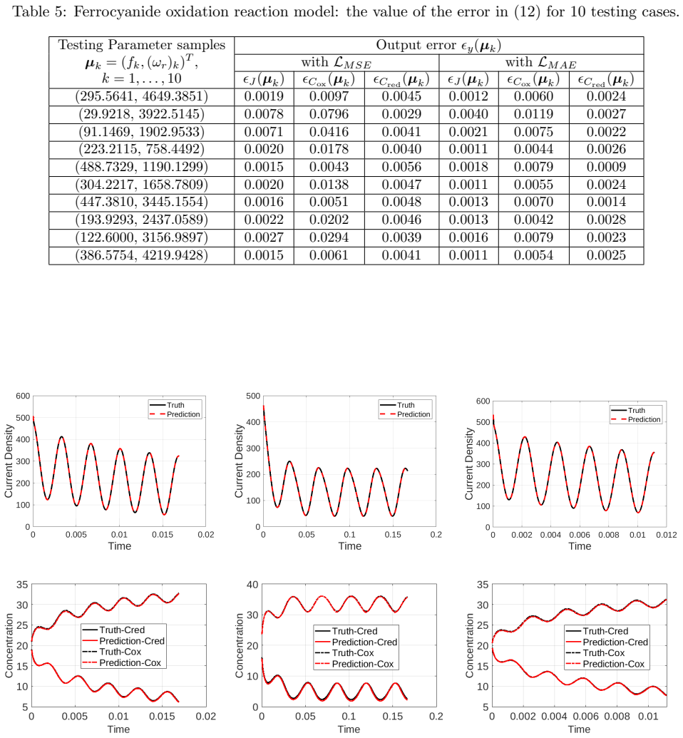
The central discovery is that reshaping the training table so that the $n_o$ output components at each time step occupy a contiguous block of length $n_o$ turns the temporal fusion transformer into a multi-output predictor, and that masking the attention matrix block-wise preserves and extends interpretability. In the block-wise masked attention matrix $\tilde{A}$, every entry $\tilde{a}_{k,l}$ inside the block for time $t_i$ encodes the correlation between output $k$ at $t_i$ and output $l$ at $t_j$, while blocks for future times are masked out as usual. With this single matrix, the model captures both temporal dependence within each output and spatial dependence across outputs, and the variable-selection layer still reports which parameters, past inputs, and past outputs drive the prediction. The paper reports that the overwhelming majority of the chaotic Lorenz-63 test cases, up to about 97 percent, were predicted with error below 5 percent, and that the mean prediction errors for the FitzHugh-Nagumo and Ferrocyanide outputs are mostly in the range of roughly 0.1 to 3 percent when the MAE loss is used, with the MAE loss consistently matching or beating the MSE loss. The paper takes these results as evidence that the approach predicts accurately regardless of system nonlinearity and the dimensionality of the parameter space.
Load-bearing premise
The method assumes that the output vector at the initial time, together with the parameters and the known future input, is a sufficient statistic for the whole future output sequence; this holds in the paper's examples only because Lorenz-63's outputs are the full state and the other two models start from fixed zero initial conditions.
Editorial extensions
If this is right
- One trained iSTFT model replaces a separate TFT model for each quantity of interest, so systems with many outputs no longer require retraining per output.
- At test time, only the initial output vector, the parameters, and the known future input are needed; the whole future output sequence is produced in one forward pass, with the three examples taking about 4 to 6.4 seconds for all test cases combined.
- The block-wise attention matrix gives a readout of which outputs are coupled and which past values matter most, information that the original single-output TFT cannot show.
- The equivalence of the $q=0.5$ quantile loss and the MAE loss means the interpretable multi-horizon forecasting framework can be used directly for accurate point predictions, not only for quantile forecasts.
Reading between the lines
- If iSTFT is applied to systems whose output is only a partial observation of the state, the initial output vector is generally not a sufficient statistic; the natural repair is to feed a short past window of outputs as observed inputs, and this window length would become a new hyperparameter.
- The learned block-wise attention weights could be read as a data-driven coupling matrix for the output variables, offering a justification for decoupling some outputs in reduced-order modeling or sensor placement decisions.
- A direct testable extension would compare iSTFT against an LSTM or neural-operator baseline on a system with hidden state but identical initial outputs, which would isolate whether the one-step multi-output property survives partial observability.
- Because the discrepancy between attention weights for different outputs was visible in the Ferrocyanide example, where the current density appeared decoupled from the concentrations, similar inspection could be used to detect output groups that evolve almost independently, guiding divide-and-conquer surrogates.
Signed reviews
Editorial analysis
A structured set of objections, weighed in public.
Referee Report
Summary. The paper proposes iSTFT, a multi-output extension of the Temporal Fusion Transformer for predicting output time series of parametric dynamical systems with time-varying inputs. The main technical ingredients are a data reshaping that aligns multiple outputs into one spatial-temporal sequence and a block-wise masked interpretable multi-head attention that couples outputs while preserving causality. The authors prove that the L1 loss is equivalent to the q=0.5 quantile loss, then evaluate on Lorenz-63 with random initial conditions, a FitzHugh-Nagumo PDE with two parameters and an external input, and a Ferrocyanide reaction model with two parameters. Reported average errors are low (for example, mean errors of 0.0066 and 0.0014 for the FitzHugh-Nagumo outputs under the MAE loss). The abstract, however, claims accuracy regardless of nonlinearity and parameter-space dimensionality, a claim not supported by the experiments.
Significance. If the central claims held, the method would be a useful non-intrusive surrogate for multi-output parametric systems. The extension of TFT's single averaged attention matrix to a block-wise spatial-temporal attention matrix is a reasonable and potentially interpretable architectural choice. The manuscript is transparent about hyperparameters and includes a formal, if elementary, proof of the loss equivalence. The three test problems cover a chaotic ODE and two nonlinear PDE-derived systems with external inputs, which is a sensible initial test bed. However, because no baselines are run and the identifiability of the prediction map from the initial output is not addressed, the demonstrated significance is substantially narrower than the abstract claims; the contribution is an incremental architecture/data-format extension whose general validity remains unproven.
major comments (4)
- [§2.1, Eq. (1); §4.3; §5] The one-step prediction setup is only well-posed if (y(t1,μ), μ, future input) uniquely determines all future outputs. Eq. (1) defines the initial condition as x(0,μ) in R^N, but the model receives only y(t1,μ)=C(μ)x(t1,μ). Section 4.1 avoids the issue because y is the full state; Section 4.2 avoids it because the initial state is fixed at zero. Section 4.3 has N=2003 and n_o=3 and provides no observability or unique-state argument. For a generic parametric system with hidden state and variable initial conditions, two different states with the same observed output at t1 can lead to different future outputs, so no transformer can be accurate in general. The abstract's claim 'regardless of ... dimensionality of the parameter space' and Section 5's statement that 'only the initial condition is needed' therefore overstate the demonstrated scope. Please either prove or assume an identifiability condition, test on a system with unobserved state and varying initial state, or restrict the claims.
- [§4.1–§4.3] The numerical evaluation contains no baselines. The introduction motivates the work by limitations of LSTM and single-output TFT, and the contribution is an architectural change; yet the paper reports only iSTFT's own errors. Without comparing to retrained single-output TFT models, an LSTM baseline, or a standard multivariate forecaster, the claimed advantage in accuracy and interpretability is not established. Please add baseline comparisons and an ablation that removes the block-wise mask.
- [Abstract; §4] The claim that accuracy holds 'regardless of ... the dimensionality of the parameter space' is not supported by any experiment with p>2; all three examples have p=2, and Lorenz-63 has random initial-condition parameters but no physical parameters or external input. Please add a higher-dimensional parameter experiment or replace the claim with a qualified statement about the tested regime.
- [§4.4] The interpretability analysis is qualitative: it relies on visual inspection of a few attention matrices and variable-importance tables, with no quantitative metric, statistical test, or comparison to an alternative attention mechanism. Since interpretability is a stated main contribution, the current evidence is anecdotal and should be either strengthened or presented as preliminary.
minor comments (6)
- [Title / Abstract] The manuscript uses two different titles, and the acronym 'SE-TFT' appears in the abstract while the body uses 'iSTFT'; please unify the naming.
- [Eq. (12)] The error measure switches discontinuously between absolute error and relative error exactly at mean |y|=1, which can make averaged errors across different outputs or examples incomparable.
- [§4.2] The text says the outputs at the 'following 500 time instances' are predicted, but only 499 future time instances follow t1; the wording is internally inconsistent.
- [Eq. (2)] The notation mixes n_μ, n_p, and n_µ in the data table; please standardize the symbol for the number of parameter samples.
- [General] No code or data availability statement is provided; for reproducibility, please include one.
- [§5] The sentence 'so that if can be used' appears to be a typo for 'so that it can be used'.
Circularity Check
No significant circularity: the reported predictions are genuine held-out generalization, and the paper's only real weakness is an overbroad applicability claim, not a circular derivation.
full rationale
The paper's contribution is an empirical architecture: it reshapes multi-output data into a single output column (Eq. 3), applies a block-wise masked attention (Sec. 3.2), and trains on data split by parameter ID (Sec. 3.3). The reported accuracies are measured on held-out parameter samples (Tables 3 and 5; Lorenz-63 testing cases 512), so no test output is used to fit a parameter. Theorem 3.1 proves L1 loss equals quantile loss at q=0.5 by elementary algebra; this equivalence is standard, is not used as an input to the model, and is not presented as a fitted result. Citations to prior work by the same authors (e.g., [43]) occur only in literature surveys and as examples of LSTM-based approaches; none is load-bearing for the iSTFT design or for the numerical claims. The one substantive weakness is that the abstract's claim of accuracy 'regardless of nonlinearity... and dimensionality of the parameter space' is broader than the demonstrated setup, since accurate one-step prediction requires y(t1), mu, and the future input signal to determine the future output trajectory; this holds in the tested examples only when the output is the full state or the initial state is fixed. That is an unstated modeling restriction and an over-generalization risk, not a circular derivation. No equation or result reduces by construction to a fitted constant, to a self-citation, or to its own input, so the circularity score is 0.
Assumptions & free parameters
free parameters (8)
- Learning rate (Lorenz / FHN / Ferro) =
0.001 / 0.0005 / 0.0005
- Model width d_model =
160
- Number of attention heads =
4 / 1 / 4
- Minibatch size =
256 / 64 / 64
- Max gradient norm =
1.0 / 100 / 0.01
- Dropout rate =
0.2 / 0.1 / 0.2
- Number of training subsets per trajectory (Lorenz) =
8
- Error-metric threshold in Eq. (12) =
1.0
assumptions (4)
- domain assumption Trained transformer generalizes to unseen parameter samples drawn from the same sampling distribution.
- domain assumption Initial output vector, parameters, and future inputs are a sufficient statistic for future outputs.
- domain assumption Numerical reference solutions are accurate ground truth.
- standard math TFT building blocks function as described in [32] and [45].
Cite this review
Pith. "Pith review of Spatially-Enhanced Temporal Fusion Transformer: Interpretable Multi-Output Prediction for Parametric Dynamical Systems with Time-Varying Inputs." pith.science (2026). https://pith.science/paper/FAZB2YL5
@misc{pith2026250500473,
  author       = {Pith},
  title        = {Pith review of: Spatially-Enhanced Temporal Fusion Transformer: Interpretable Multi-Output Prediction for Parametric Dynamical Systems with Time-Varying Inputs},
  year         = {2026},
  howpublished = {\url{https://pith.science/paper/FAZB2YL5}},
  note         = {Machine review of arXiv:2505.00473}
}
read the original abstract
We explore the promising performance of a transformer model in predicting outputs of parametric dynamical systems with external time-varying input signals. The outputs of such systems vary not only with physical parameters but also with external time-varying input signals. Accurately catching the dynamics of such systems is challenging. We have adapted and extended an existing transformer model, called temporal fusion transformer (TFT), for single-output prediction to a multiple-output transformer, named as Spatially-Enhanced Temporal Fusion Transformer (SE-TFT), which is able to predict multiple output responses of these systems. The SE-TFT generalizes the interpretability of the original TFT model. The generalized interpretable attention weight matrix explores not only the temporal correlations in the sequence, but also the interactions between the multiple outputs, providing explanation for the spatial correlation in the output domain. This proposed SE-TFT accurately predicts the sequence of multiple outputs, regardless of the nonlinearity of the system and the dimensionality of the parameter space.
Figures


Figures from the paper (9 more)




Reference graph
Works this paper leans on
-
[1]
A. C. Antoulas. Approximation of Large-Scale Dynamical Systems, volume 6 of Adv. Des. Control. SIAM Publications, Philadelphia, PA, 2005
work page 2005
-
[2]
J. Barnett and C. Farhat. Quadratic approximation manifold for mitigating the kolmogorov barrier in nonlinear projection-based model order reduction. J. Comput. Phys., 464:111348, 2022
work page 2022
-
[3]
J. Barnett, C. Farhat, and Y. Maday. Neural-network-augmented projection-based model order reduction for mitigating the kolmogorov barrier to reducibility. J. Comput. Phys. , 492:112420, 2023
work page 2023
-
[4]
J. Beitner and F. Kiraly. Pytorch forecasting. https://github.com/sktime/ pytorch-forecasting, 2020. Accessed: 2025-04-29
work page 2020
- [5]
- [6]
- [7]
- [8]
Show all 51 references
-
[9]
Bonneville, Y
C. Bonneville, Y. Choi, D. Ghosh, and J. L. Belof. gpLaSDI: Gaussian process-based interpretable latent space dynamics identification through deep autoencoder. Comp. Meth. Appl. Mech. Eng. , 418:116535, 2024
2024
-
[10]
Calvello, N
E. Calvello, N. B. Kovachki, M. E. Levine, and A. M. Stuart. Continuum attention for neural operators. arxiv e-prints: 2406.06486, 2024. cs.LG
2024
-
[11]
Chellappa, L
S. Chellappa, L. Feng, V. de la Rubia, and P. Benner. Inf-sup-constant-free state error estimator for model order reduction of parametric systems in electromagnetics. IEEE Trans. Microw. Theory Techn., 2023
2023
-
[12]
R. T. Q. Chen, Y. Rubanova, J. Bettencourt, and D. K. Duvenaud. Neural ordinary differential equations. In Advances in Neural Information Processing Systems , volume 31, page 6572–6583. Curran Associates, Inc., 2018
2018
-
[13]
Cirstea, C
R. Cirstea, C. Guo, B. Yang, T. Kieu, X. Dong, and S. Pan. Triformer: Triangular, Variable- Specific Attentions for Long Sequence Multivariate Time Series Forecasting. In L. D. Raedt, editor, Proceedings of the Thirty-First International Joint Conference on Artificial Intellig...
1994
-
[14]
Conti, G
P. Conti, G. Gobat, S. Fresca, A. Manzoni, and A. Frangi. Reduced order modeling of parametrized systems through autoencoders and SINDy approach: continuation of periodic solu- tions. Comp. Meth. Appl. Mech. Eng. , 411:116072, 2023
2023
-
[15]
Conti, M
P. Conti, M. Guo, A. Manzoni, and J. S. Hesthaven. Multi-fidelity surrogate modeling using long short-term memory networks. Comp. Meth. Appl. Mech. Eng. , 404:115811, 2023. 21
2023
-
[16]
Drouin, E
A. Drouin, E. Marcotte, and N. Chapados. TACTiS: Transformer-Attentional Copulas for Time Series. In K. Chaudhuri, S. Jegelka, L. Song, C. Szepesvari, G. Niu, and S. Sabato, editors, Proceedings of the 39th International Conference on Machine Learning, volume 162 of Proceeding...
2022
-
[17]
Dutta, M
S. Dutta, M. W. Farthing, E. Perracchione, G. Savant, and M. Putti. A greedy non-intrusive reduced order model for shallow water equations. J. Comput. Phys. , 439:110378, 2021
2021
-
[18]
Feldmann and R
P. Feldmann and R. W. Freund. Efficient linear circuit analysis by Pad´ e approximation via the Lanczos process. IEEE Trans. Comput.-Aided Design Integr. Circuits Syst. , 14:639–649, 1995
1995
-
[19]
L. Feng. Predicting output responses of nonlinear dynamical systems with parametrized inputs using LSTM. IEEE J. Multiscale Multiphysics Comput. Tech. , 8:97–107, 2023
2023
-
[20]
FitzHugh
R. FitzHugh. Impulses and physiological states in theoretical models of nerve membrane. Biophys. J., 1(6):445–466, 1961
1961
-
[21]
Fresca, L
S. Fresca, L. Ded` e, and A. Manzoni. A comprehensive deep learning-based approach to reduced order modeling of nonlinear time-dependent parametrized PDEs. J. Sci. Comput. , 87:61, 2021
2021
-
[22]
Fresca and A
S. Fresca and A. Manzoni. POD-DL-ROM: Enhancing deep learning-based reduced order models for nonlinear parametrized PDEs by proper orthogonal decomposition. Comp. Meth. Appl. Mech. Eng., 388:114181, 2022
2022
-
[23]
Geneva and N
N. Geneva and N. Zabaras. Transformers for modeling physical systems. Neural Networks , 146:272–289, 2022
2022
-
[24]
Z. Hao, Z. Wang, H. Su, C. Ying, Y. Dong, S. Liu, Z. Cheng, J. Song, and J. Zhu. GNOT: A general neural operator transformer for operator learning. In A. Krause, E. Brunskill, K. Cho, B. Engelhardt, S. Sabato, and J. Scarlett, editors, Proceedings of the 40th International Con...
2023
-
[25]
X. He, Y. Choi, W. D. Fries, J. L. Belof, and J.-S. Chen. gLaSDI: Parametric physics-informed greedy latent space dynamics identification. J. Comput. Phys. , 489:112267, 2023
2023
-
[26]
J. S. H. J. Duan. Non-intrusive data-driven reduced-order modeling for time-dependent parametrized problems. J. Comput. Phys. , 497:112621, 2024
2024
-
[27]
M. Kast, M. Guo, and J. S. Hesthaven. A non-intrusive multifidelity method for the reduced order modeling of nonlinear problems. Comp. Meth. Appl. Mech. Eng. , 364, 2020
2020
-
[28]
Kontolati, S
K. Kontolati, S. Goswami, G. E. Karniadakis, and M. D. Shields. Learning nonlinear operators in latent spaces for real-time predictions of complex dynamics in physical systems. Nat. Commun., 15(1):5101, 2024
2024
-
[29]
J. N. Kutz. Machine learning methods for reduced order modeling. In M. Falcone and G. Rozza, editors, Model Order Reduction and Applications, volume 2328 of Lecture Notes in Mathematics, pages 201–228. Springer Cham., 2021
2021
-
[30]
Z. Li, N. Kovachki, K. Azizzadenesheli, B. Liu, K. Bhattacharya, A. Stuart, and A. Anandkumar. Fourier Neural Operator for parametric partial differential equations. arxiv e-prints: 2010.08895,
2010 arXiv
-
[31]
Z. Li, N. Kovachki, K. Azizzadenesheli, B. Liu, A. Stuart, and A. Anandkumar. Neural Operator: Graph Kernel Network for Partial Differential Equations. arxiv e-prints: 2003.03485, 2020. cs.LG
2003 arXiv
-
[32]
B. Lim, S. O. Arık, N. Loeff, and T. Pfister. Temporal Fusion Transformers for interpretable multi-horizon time series forecasting. Int. J. Forecast., 37(4):1748–1764, 2021
2021
-
[33]
Y. Lin, I. Koprinska, and M. Rana. SSDNet: State Space Decomposition Neural Network for Time Series Forecasting . In 2021 IEEE International Conference on Data Mining (ICDM) , pages 370–378, 2021
2021
-
[34]
Y. Liu, H. Wu, J. Wang, and M. Long. Non-stationary transformers: exploring the stationarity in time series forecasting. In Proceedings of the 36th International Conference on Neural Information Processing Systems, NIPS ’22. Curran Associates Inc., 2024
2024
-
[35]
L. Lu, P. Jin, G. Pang, Z. Zhang, and G. E. Karniadakis. Learning nonlinear operators via Deep- ONet based on the universal approximation theorem of operators. Nat. Mach. Intell. , 3(3):218– 229, 2021
2021
-
[36]
Maulik, B
R. Maulik, B. Lusch, and P. Balaprakash. Reduced-order modeling of advection-dominated systems with recurrent neural networks and convolutional autoencoders. Physics of Fluids , 33(3):037106, 2021
2021
-
[37]
Moradi A., S
M. Moradi A., S. A. Sadrossadat, and V. Derhami. Long short-term memory neural networks for modeling nonlinear electronic components. IEEE Trans. Compon. Packag. Technol. , 11(5):840– 847, 2021
2021
-
[38]
Ovadia, A
O. Ovadia, A. Kahana, P. Stinis, E. Turkel, D. Givoli, and G. E. Karniadakis. ViTO: Vision Transformer-Operator. Comp. Meth. Appl. Mech. Eng. , 428:117109, 2024
2024
-
[39]
L. T. Pillage and R. A. Rohrer. Asymptotic waveform evaluation for timing analysis. IEEE Trans. Comput.-Aided Design Integr. Circuits Syst. , 9(4):352–366, 1990
1990
-
[40]
Shabani, A
A. Shabani, A. Abdi, L. Meng, and T. Sylvain. Scaleformer: Iterative multi-scale refining trans- formers for time series forecasting. In The Eleventh International Conference on Learning Rep- resentations, 2023
2023
-
[41]
Shen and Y
L. Shen and Y. Wang. TCCT: Tightly-coupled convolutional transformer on time series forecast- ing. Neurocomputing, 480:131–145, 2022
2022
-
[42]
Solera-Rico1, C
A. Solera-Rico1, C. S. Vila1, M. A. G´ omez, Y. Wang, A. Almashjary, S. T. M. Dawson, and R. Vinuesa. β-variational autoencoders and transformers for reduced-order modelling of fluid flows. Nat. Commun., 15(1):1361, 2024
2024
-
[43]
S. Sun, L. Feng, and P. Benner. Data-Augmented Predictive Deep Neural Network: Enhancing the extrapolation capabilities of non-intrusive surrogate models. arxiv e-prints:2410.13376, 2024. cs.LG
2024 arXiv
-
[44]
Fitzhugh-nagumo system
The MORwiki Community. Fitzhugh-nagumo system. http://modelreduction.org/index. php/FitzHugh-Nagumo_System, 2018
2018
-
[45]
Vaswani, N
A. Vaswani, N. Shazeer, N. Parmar, J. Uszkoreit, L. Jones, A. N. Gomez, L. Kaiser, and I. Polo- sukhin. Attention is all you need. In Proceedings of the 31st International Conference on Neural Information Processing Systems, NIPS’17, page 6000–6010. Curran Associates Inc., 2017. 23
-
[46]
Vidakovi´ c-Koch, V
T. Vidakovi´ c-Koch, V. Pani´ c, M. Andri´ c, M. Petkovska, and K. Sundmacher. Nonlinear frequency response analysis of the ferrocyanide oxidation kinetics. part I. a theoretical analysis. J. Phys. Chem. C, 115(8):17341–17351, 2011
2011
-
[47]
Q. Wen, T. Zhou, C. Zhang, W. Chen, Z. Ma, J. Yan, and L. Sun. Transformers in time series: A survey. In Proceedings of the Thirty-Second International Joint Conference on Artificial Intelligence, 2023
2023
-
[48]
N. Wu, B. Green, X. Ben, and S. O’Banion. Deep transformer models for time series forecasting: The influenza prevalence case. arxiv e-prints: 2001.08317, Jan. 2020. cs.LG
2001 arXiv
-
[49]
Zhang and J
Y. Zhang and J. Yan. Crossformer: Transformer utilizing cross-dimension dependency for multi- variate time series forecasting. In The Eleventh International Conference on Learning Represen- tations, 2023
2023
-
[50]
H. Zhou, S. Zhang, J. Peng, S. Zhang, J. Li, H. Xiong, and W. Zhang. Informer: Beyond efficient transformer for long sequence time-series forecasting. In The Thirty-Fifth AAAI Conference on Artificial Intelligence, AAAI 2021, Virtual Conference , volume 35, pages 11106–11115. ...
2021
-
[51]
T. Zhou, Z. Ma, Q. Wen, X. Wang, L. Sun, and R. Jin. FEDformer: Frequency enhanced decomposed transformer for long-term series forecasting. In Proceedings of the 39th International Conference on Machine Learning (PMLR) , volume 162, pages 27268–27286, 2022. 24
2022
Reviewed August 16, 2026 · model on record in the stance chip above.
Discussion (0). Continue with ORCID to comment.