REVIEW 2 major objections 6 minor 1 cited by
Q-ball perturbations with more details: linear analysis vs lattice
T0 review · 2 major / 6 minor · reviewed 2026-08-11 · deepseek-v4-flash
Pith's one-line read This paper shows linear Q-ball perturbation theory is valid up to ~1% amplitude and that energy extraction requires opposite-charge incoming particles.
desk verdict Careful linear-vs-lattice study of Q-ball perturbations; the δr bound is plausible but needs the missing numerical details before it is fully established. read the letter →
The pith
A machine-rendered reading of the paper's core claim, the machinery that carries it, and where it could break.
The reading
What carries the argument
The load-bearing object is the conserved particle-number current $J_\eta = 2\,\mathrm{Im}\left(\eta_+^*\nabla\eta_+ - \eta_-^*\nabla\eta_-\right)$ (extended to $J_\eta = 2\,\mathrm{Im}(\eta_\chi\nabla\eta_\chi^* + \eta_+\nabla\eta_+^* - \eta_-\nabla\eta_-^*)$ in the two-field model), whose conservation makes the scattering matrix $S$ unitary; because the linearized equations are real, $S$ is also symmetric, and the transformation $\omega \to -\omega$ swaps the $\eta_+$ and $\eta_-$ modes. These three properties fix the transition probabilities up to a few real parameters and let the paper deduce the selection rule that only an opposite-charge incoming mode can reduce the Q-ball's energy. The amplification factors $Z_E$ and $Z_Q$ are then defined from the asymptotic fluxes, and the paper shows $Z_E$ for the antiparticle channel equals the ratio $|A^{\mathrm{out}}_+|^2 (E(Q)-E(Q-2))/|\omega_-|$, up to subleading terms suppressed by $d^2 E/dQ^2$.
What would settle it
Repeat the one-field scattering for $\delta r = 10^{-2}$ at two grid spacings that differ by a factor of two and with the absorbing boundary moved twice as far away; if the extracted $Z_E$ and $Z_Q$ change by more than the tolerance that currently separates the linear and lattice curves, the claimed validity domain is a numerical artifact rather than a statement about the continuum theory.
Extended reading notes
Core claim
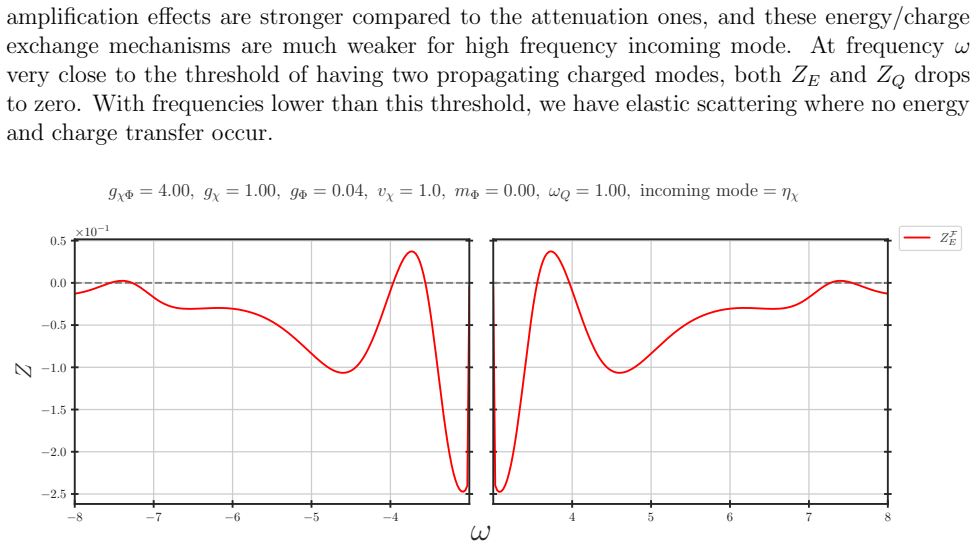
On the paper's own terms, the central discovery is that the flux-based amplification factors $Z_E$ and $Z_Q$ computed from the linearized perturbation equations agree with full nonlinear lattice simulations once the perturbation size is below $\delta r \lesssim 10^{-2}$, where $\delta r$ is the rescaled amplitude of the incoming wave packet relative to the Q-ball field value. For such small perturbations the conserved current $J_\eta$ and the symmetric unitary $S$-matrix relating incoming and outgoing mode amplitudes provide an exact description of charge and energy exchange. The paper also establishes, by matching the amplification factor to the Q-ball self-energy difference, that energy extraction requires an incoming antiparticle mode $\eta_-$ for a positive-charge Q-ball, and that in the two-field FLS model all three modes ($\eta_+$, $\eta_-$, $\eta_\chi$) mix, so energy exchange proceeds through reactions with three distinct energies.
Load-bearing premise
The load-bearing premise is that the lattice simulations faithfully reproduce the continuum nonlinear dynamics: the absorbing boundary must not contaminate the measured fluxes, the fourth-order finite-difference and Runge-Kutta discretization must be converged, and the initial Q-ball profile must be accurate enough that its spurious radiation is negligible compared with the signals it contaminates.
Editorial extensions
If this is right
- For perturbation sizes $\delta r \lesssim 10^{-2}$, energy and charge exchange between a Q-ball and surrounding plasma can be computed reliably from linear scattering theory, which directly feeds solitosynthesis rate estimates.
- At early-universe temperatures roughly an order of magnitude below the mass scale $\mu$, the linear regime is realized; for non-relativistic plasma particles the dominant processes are elastic scattering or a reduction of the Q-ball charge.
- The selection rule means a positively charged Q-ball can lose energy and charge only through collisions with antiparticles $\phi^\dagger$; same-sign particles can only add energy and charge.
- In the FLS two-field model, a neutral $\chi$ quantum can either release or absorb energy depending on its frequency, and the three-mode structure opens the channel $Q + \chi \to (Q-1) + \phi$ alongside the charged channels.
Reading between the lines
- Editorial: the $\delta r \lesssim 10^{-2}$ validity threshold is established for the specific one-field potential with $g=1/3$ and spherical waves; the same threshold may shift for thin-walled Q-balls or for high angular momentum, a testable extension of the paper's lattice comparison.
- Editorial: the exactness of the selection rule (energy extraction only from opposite-charge quanta) is a linear-order statement; at nonlinear amplitudes $\delta r > 10^{-2}$ the paper's own simulations show the Q-ball deforms and oscillates, so the rule should not be extrapolated to strong scattering.
- Editorial: the conserved-current argument implies an exact all-order (in $\omega$ but linear in amplitude) statement about elastic scattering of half-propagating modes; since $|A^{\mathrm{in}}_+|^2 = |A^{\mathrm{out}}_+|^2$, a Q-ball that is classically forbidden to lose charge at low energies will show this behavior sharply at the threshold, which could be probed in a single-mode wave-packet expe
- Editorial: the FLS three-mode mixing suggests a mediator-catalyzed process in which a neutral $\chi$ background can convert a same-sign charged quantum into an opposite-sign one, effectively flipping the sign of energy exchange; whether this enhances or suppresses net charge accretion in a plasma is not addressed by the paper.
Editorial analysis
A structured set of objections, weighed in public.
Referee Report
Summary. The paper studies the linear response of non-rotating Q-balls in a one-complex-field model and in an FLS two-field model. It derives a conserved particle-number current, encodes the scattering in a symmetric unitary S-matrix, and obtains charge/energy amplification factors for S-wave and higher partial waves. The authors compare linear predictions with full nonlinear lattice simulations and conclude that linear analysis remains valid for perturbations δr ≲ 10^-2, with applications to solitosynthesis in the early universe. The FLS analysis, including a three-mode conserved current and energy extraction channels, is presented as new.
Significance. The analytic machinery—conserved current, S-matrix symmetries, and the flux definitions—is derived cleanly and contains no free parameters; the energy-balance consistency check in Eqs. (24)–(26) is a useful independent cross-check, and the lattice comparison is a meaningful test of the linear approximation. If the numerical evidence is supplied, the paper would establish a practical validity criterion for solitosynthesis calculations and provide the first linear/lattice treatment of FLS Q-ball perturbation scattering. The early-universe estimate in Section 2.3 is a suggestive but tentative application.
major comments (2)
- [Sec. 2.2–2.3, Fig. 6] The quantitative threshold δr ≲ 10^-2 is the paper's headline validity claim and rests entirely on the lattice-vs-linear comparison, yet no lattice parameters are reported: no grid spacing Δx, time step Δt, boundary radius, absorbing-boundary specification, or convergence test. The manuscript itself lists "discretisation of time and space leading to the generic systematic error" and the requirement that the initial Q-ball profile be exact, otherwise radiation becomes a background. With a 4th-order finite-difference scheme, O(Δx^4) errors and spurious Q-ball radiation could mimic the physical nonlinear corrections at δr ~ 10^-2; therefore the claim is not established until the lattice data are shown to converge and to be background-free. The same numerical-detail deficit applies to the two-field comparison in Fig. 20.
- [Sec. 3, Eq. (62)] The energy-amplification formula for the two-field model is internally inconsistent in its mode labels. The text assumes an initial η− state, but the displayed definitions set A_in_+ = 1 and A_in_- = 0, which describe an incoming η+ state. With the paper's flux definition in Eq. (21), an η− initial state gives 1+Z_Q = |A_out_-|^2 − |A_out_+|^2 (up to the absolute value), not |A_out_+|^2 − |A_out_-|^2. The sign and mode content of Eq. (62), and hence the derived two-field energy-extraction selection rule, need to be corrected.
minor comments (6)
- [Sec. 2] There is a typo "various vaious" in the opening of Section 2; please correct it.
- [Figs. 8, 15–20] The η− mode is rendered as a square or "□" symbol in several figures, presumably due to a missing glyph; please use the same notation as in the text.
- [Appendix C.2] The two-field perturbation is specified by δ_Φ = 5×10^-4 and σ_Φ = 10, but it is not mapped to the δr variable defined in Eq. (43), so the reader cannot compare the two-field lattice agreement with the one-field threshold.
- [Sec. 2.3, Eqs. (44)–(45)] The identification of the wavepacket coherence length with the inverse plasma temperature is an assumption that should be stated explicitly as a modeling choice, with a short justification or a caveat about its range of validity.
- [Appendix A, Eq. (77)] Equation (77) contains a repeated identical expression on both sides of the equality; the intended limit statement should be written out.
- [Abstract] The phrase "as well discussion of the FLS Q-balls" should read "as well as a discussion of the FLS Q-balls".
Circularity Check
No significant circularity: the linear predictions, lattice validations, and kinematic energy-balance checks are independent computations with no fitted parameters passed between them.
full rationale
The central derivation chain is self-contained and does not reduce to its own inputs. The linear perturbation results follow from solving the fixed Q-ball profile equations (Eqs. (10) and (53)) with no free parameters; the charge and energy amplification factors in Eq. (21) are defined directly from asymptotic scattering amplitudes. The lattice comparisons in Figs. 6 and 20 compute the same flux ratios from independent nonlinear evolution with the initial conditions of Eqs. (36)-(37), using no fitted values taken from the linear calculation. The kinematic energy-extraction estimate in Eq. (23) is explicitly presented as a consistency check: it combines the linear transition probability |Aout_+|^2 with the Q-ball binding-energy difference E(Q)-E(Q-2), and Eqs. (24)-(26) show that this reduces to the flux-based ZE through the standard identity dE/dQ = omega_Q, up to higher-derivative corrections. This is a derived consistency relation, not an input used to construct the linear result. The selection rule that energy extraction from a positive-charge Q-ball requires an incoming antiparticle follows from charge conservation together with the monotonicity of E(Q), and is corroborated by the mode-energy ordering of Eq. (28); it is not definitionally identical to the amplification factors being predicted. The FLS three-mode analysis is an extension obtained by linearizing the two-field equations of motion and defining the conserved current of Eq. (54); no uniqueness theorem or author-imported ansatz is used to force the result. The cited prior works [23,24] are by other authors and serve only as starting points, not as load-bearing self-citations. The paper's quantitative claim that linear analysis remains valid up to delta_r ≲ 10^-2 rests on lattice comparisons whose grid spacing, time step, and convergence behavior are not reported; this is a missing-support or correctness concern, not circularity, because the lattice computation is an independent check rather than a fitted input. No circular step can be exhibited from the paper's own equations.
Assumptions & free parameters
assumptions (6)
- domain assumption Q-ball profile is the spherically symmetric classical solution satisfying Eq. (5) with boundary conditions ϕ'Q(0)=0 and ϕQ(∞)=0.
- domain assumption Perturbations admit the two-frequency ansatz Φ1 = η+ e^{-iω+ t} + η- e^{-iω- t}, with ω± = ωQ ± ω, and bound modes are excluded except where stated.
- standard math The S-matrix is unitary and symmetric due to current conservation and reality of the linear operator O(r).
- domain assumption Lattice discretization with 4th-order finite differences and RK4 converges to the continuum solution, and absorbing boundaries do not contaminate flux measurements.
- domain assumption Classical wavepacket scattering amplitudes can be interpreted as quantum transition probabilities for single particles, with reactions listed in Eq. (22).
- ad hoc to paper Early-universe plasma quanta can be modeled as coherent wavepackets of charge Q=1 and size of order inverse temperature, as used in Eqs. (44)-(45).
Cite this review
Pith. "Pith review of Q-ball perturbations with more details: linear analysis vs lattice." pith.science (2026). https://pith.science/paper/FFDEZC3S
@misc{pith2026241213885,
  author       = {Pith},
  title        = {Pith review of: Q-ball perturbations with more details: linear analysis vs lattice},
  year         = {2026},
  howpublished = {\url{https://pith.science/paper/FFDEZC3S}},
  note         = {Machine review of arXiv:2412.13885}
}
read the original abstract
We analyze in detail the interactions between non-topological soliton (Q-ball) and its perturbations. We extend the previous literature by carefully identifying the domain of applicability of linear analysis as well discussion of the FLS Q-balls. Applications to the early universe physics are briefly commented.
Figures


Figures from the paper (17 more)




Forward citations
Cited by 1 Pith paper
-
Oscillon Floquet Modes and the Operators that Excite Them
Relativistic Floquet modes of the oscillon are expressed in elementary functions, and their quantum creation/annihilation operators are shown to satisfy the oscillator algebra at the computed order.
Reference graph
Works this paper leans on
-
[1]
S. R. Coleman Phys. Rev. D15 (1977) 2929–2936. [Erratum: Phys. Rev.D16,1248(1977)]. 2
work page 1977
-
[2]
R. Friedberg, T. D. Lee, and A. Sirlin Nucl. Phys. B115 (1976) 32–47. 2, 13
work page 1976
-
[3]
R. Friedberg, T. D. Lee, and A. Sirlin Nucl. Phys. B115 (1976) 1–31. 2, 13
work page 1976
-
[4]
R. Friedberg, T. D. Lee, and A. Sirlin Phys. Rev. D13 (1976) 2739–2761. 2, 7, 13
work page 1976
-
[5]
T. D. Lee and Y. Pang Phys. Rept. 221 (1992) 251–350. 2, 7, 13
work page 1992
-
[6]
E. Y. Nugaev and A. V. Shkerin J. Exp. Theor. Phys.130 (2020), no. 2 301–320, [ arXiv:1905.05146]. 2
arXiv 2020
-
[7]
A. Kusenko and M. E. Shaposhnikov Phys. Lett. B418 (1998) 46–54, [ hep-ph/9709492]. 2
arXiv 1998
- [8]
Show all 35 references
-
[9]
Enqvist and J
K. Enqvist and J. McDonald Phys. Lett. B440 (1998) 59–65, [ hep-ph/9807269]. 2
1998 arXiv
-
[10]
Kusenko and P
A. Kusenko and P. J. Steinhardt Phys. Rev. Lett.87 (2001) 141301, [ astro-ph/0106008]. 2
2001 arXiv
-
[11]
Roszkowski and O
L. Roszkowski and O. Seto Phys. Rev. Lett.98 (2007) 161304, [ hep-ph/0608013]. 2
2007 arXiv
-
[12]
I. M. Shoemaker and A. Kusenko Phys. Rev. D80 (2009) 075021, [ arXiv:0909.3334]. 2
2009 arXiv
-
[13]
Kasuya and M
S. Kasuya and M. Kawasaki Phys. Rev. D84 (2011) 123528, [ arXiv:1107.0403]. 2
2011 arXiv
-
[14]
Kasuya, M
S. Kasuya, M. Kawasaki, and M. Yamada Phys. Lett. B726 (2013) 1–7, [ arXiv:1211.4743]. 2
2013 arXiv
- [15]
-
[16]
Pont´ on, Y
E. Pont´ on, Y. Bai, and B. Jain JHEP 09 (2019) 011, [ arXiv:1906.10739]. 2, 13
2019 arXiv
-
[17]
Krylov, A
E. Krylov, A. Levin, and V. Rubakov Phys. Rev. D87 (2013), no. 8 083528, [ arXiv:1301.0354]. 2, 13
2013 arXiv
-
[18]
Bishara, G
F. Bishara, G. Johnson, O. Lennon, and J. March-Russell JHEP 11 (2017) 179, [ arXiv:1708.04620]. 2
2017 arXiv
-
[19]
J. A. Frieman, G. B. Gelmini, M. Gleiser, and E. W. Kolb Phys. Rev. Lett.60 (1988) 2101. 2
1988
-
[20]
Griest, E
K. Griest, E. W. Kolb, and A. Massarotti Phys. Rev. D40 (1989) 3529. 2
1989
-
[21]
Griest and D
K. Griest and D. Seckel Phys. Rev. D43 (1991) 3191–3203. 2
1991
- [22]
-
[23]
P. M. Saffin, Q.-X. Xie, and S.-Y. Zhou Phys. Rev. Lett.131 (2023), no. 11 111601, [ arXiv:2212.03269]. 2, 3, 5, 6, 19
2023 arXiv
-
[24]
Cardoso, R
V. Cardoso, R. Vicente, and Z. Zhong Phys. Rev. Lett.131 (2023), no. 11 111602, [ arXiv:2307.13734]. 2, 3, 5, 6, 19
2023 arXiv
-
[25]
M. N. Smolyakov Phys. Rev. D97 (2018), no. 4 045011, [ arXiv:1711.05730]. 4
2018 arXiv
- [26]
-
[27]
M. N. Smolyakov Phys. Rev. D100 (2019), no. 4 045002, [ arXiv:1906.02117]. 4
2019 arXiv
-
[28]
Heeck, A
J. Heeck, A. Rajaraman, R. Riley, and C. B. Verhaaren Phys. Rev. D103 (2021), no. 4 045008, [arXiv:2009.08462]. 7
2021 arXiv
-
[29]
Y. Bai, S. Lu, and N. Orlofsky JHEP 10 (2022) 181, [ arXiv:2208.12290]. 13
2022 arXiv
- [30]
- [31]
- [32]
-
[33]
Y. Bai, J. Berger, M. Korwar, and N. Orlofsky JHEP 10 (2021) 147, [ arXiv:2106.12589]. 13
2021 arXiv
- [34]
-
[35]
Zhang, F.-M
G.-D. Zhang, F.-M. Chang, P. M. Saffin, Q.-X. Xie, and S.-Y. Zhou arXiv:2402.03193. 22, 23 31
Reviewed August 11, 2026 · model on record in the stance chip above.
Discussion (0). Continue with ORCID to comment.