REVIEW 5 major objections 4 minor 79 references
A Blind Multiscale Spatial Regularization Framework for Kernel-based Spectral Unmixing
T0 review · 5 major / 4 minor · reviewed 2026-08-14 · deepseek-v4-flash
Pith's one-line read A two-scale spatial regularization scheme with noise-derived parameters makes kernel-based nonlinear spectral unmixing beat TV-regularized unmixing without user tuning.
desk verdict Solid kernel-unmixing paper whose real value is the multiscale regularization and dual solver; the 'truly blind' claim is overstated and the C2 derivation rests on an unvalidated uncorrelatedness assumption. read the letter →
The pith
A machine-rendered reading of the paper's core claim, the machinery that carries it, and where it could break.
The reading
What carries the argument
The central object is the multiscale transformation $W$ built from a superpixel decomposition of the image, which maps the unmixing problem into a coarse domain of roughly $K$ averaged regions and back to the fine pixel domain. The argument is carried by a statistical parameter-selection framework: assumptions A3 and A6 state that modeling errors are nearly constant within each superpixel and that the three scale-difference terms in equation (25) are mutually uncorrelated and zero-mean, which lets the authors replace the regularization constants by computable expectations involving the noise covariance $\Sigma_e$, the modeling-error variance $\sigma^2_{e,\psi}$, and the average superpixel size $S$. The optimization machinery is Lagrangian duality: the quadratically constrained primal problems are solved through their duals, whose optimality conditions reduce to root-finding equations $g_0=0$ and $g_1=g_2=0$, handled by multidimensional bisection.
What would settle it
On a real image with known endmembers, compute per-pixel residuals after fitting the linear model and a smooth kernel term, then compare the within-superpixel variance of these residuals to the total variance; if they are comparable, assumption A3 fails and the cancellation behind $C_0$ and the coarse-to-fine noise term is broken. Alternatively, estimate the sample cross-correlations among the three vectors in assumption A6; if they are not near zero, the fine-scale constraint in problem (32) is biased.
Extended reading notes
Core claim
The central claim is that a two-scale decomposition of the kernel-based mixing model improves abundance estimation precisely because the cross-scale interactions can be characterized statistically. First, superpixel averages of the image are unmixed with a coarse model, and the resulting abundances are mapped back to the full image domain. Then each pixel is unmixed subject to two equality constraints: one fixing the reconstruction-error energy to the expected noise-plus-modeling-error power $C_1$, and one fixing the abundance distance to the coarse estimate to a value $C_Y - C_E$ that corrects for the expected fine-scale noise and the nonlinear fluctuation between scales. The paper proves (Theorem 1) that strong duality holds for these nonconvex problems when the optimal Lagrangian multipliers are strictly positive, so the solutions can be obtained exactly by solving the dual as a low-dimensional root-finding problem. The authors claim this yields piecewise smooth abundance maps that preserve sharp discontinuities, and reports that it outperforms TV-regularized kernel unmixing on almost all synthetic and real benchmarks.
Load-bearing premise
The load-bearing premise is that, within each superpixel, the modeling errors of the mixing model are approximately constant across pixels, and that the three coarse-to-fine difference terms entering equation (25) are mutually uncorrelated and zero-mean.
Editorial extensions
If this is right
- Kernel-based nonlinear unmixing can exploit spatial regularity at two scales without user-set weights, because $C_0$, $C_1$ and $C_2$ follow from noise statistics rather than manual tuning.
- Piecewise smooth abundance maps that preserve sharp discontinuities become achievable with kernel methods, closing a gap that TV regularization addressed only partially.
- The strong-duality result justifies solving nonconvex quadratically constrained unmixing problems exactly through their duals, making the approach principled rather than heuristic.
- The superpixel count $K$ is selected automatically from a spectral-homogeneity criterion (ratio of leading singular values), removing another free parameter.
- Computational cost stays on the same order as TV-based kernel unmixing while removing the grid search that those methods require.
Reading between the lines
- An extension the authors leave implicit: the same two-scale consistency step could be applied to vector-valued kernel unmixing or deep feature mappings, since the correction term only requires a left inverse of the endmember matrix.
- The statistical derivation suggests a concrete diagnostic: if noise is correlated across bands, the trace terms $\operatorname{tr}\{\Sigma_e\}$ and $\|M^\dagger \Sigma_e^{1/2}\|_F^2$ should be replaced by band-weighted versions; a reader could test whether using the full covariance restores accuracy on highly correlated real noise.
- Because assumption A6 rules out correlation between abundance differences and nonlinear fluctuations, scenes with smooth illumination gradients or shade variation may violate it; measuring those cross-terms on a validation image would show how far the automatic constants can be trusted.
- The homogeneity criterion for $K$ treats each superpixel as nearly rank-1; testing it against alternative segmentation methods could reveal whether the automatic scale choice depends more on the segmentation algorithm than on the criterion itself.
Signed reviews
Editorial analysis
A structured set of objections, weighed in public.
Referee Report
Summary. The paper proposes BMUA-N, a multiscale spatial regularization framework for kernel-based nonlinear hyperspectral unmixing. The algorithm first unmixes a superpixel-coarsened image (coarse scale) and then uses the coarse abundances as prior information for the original-resolution (fine scale) problem. Both stages are formulated as quadratically constrained optimization problems with equality constraints on reconstruction error and cross-scale abundance variation. The constants C0, C1 and C2 are derived from statistical assumptions on the noise and modeling errors, so that, the authors claim, no ad hoc regularization parameter adjustment is needed. The nonconvex problems are solved through Lagrangian duality, with strong duality established in an appendix, and the dual problems are reduced to low-dimensional root-finding tasks solved by a multidimensional bisection method. Experiments on synthetic bilinear and post-nonlinear mixing models and on Cuprite, Urban and Jasper Ridge images compare BMUA-N against FCLS, K-Hype, K-Hype-TV, CDA-NL and NDU.
Significance. If the claims are correct, BMUA-N is a meaningful contribution: it provides a principled approach to setting spatial regularization constants in nonlinear unmixing, avoids user tuning of those constants, and shows competitive performance while retaining computational complexity comparable to TV-based kernel unmixing. The strong-duality argument in Appendix A is a useful contribution, and the experimental comparison is extensive, including multiple synthetic models, noise levels, real datasets and several baseline algorithms. The paper also gives a concrete method for selecting the number of superpixels from spectral homogeneity. However, the central theoretical derivation of C2 and the 'truly blind' claim rest on assumptions that are not validated and, for the bilinear and post-nonlinear models actually used in the experiments, are structurally questionable. Because those assumptions directly feed the fine-scale constraint, the main claim is not yet fully supported.
major comments (5)
- [Section IV-C, Eq. (25)] Assumption A6 is load-bearing for the derivation of C2, but it is not validated and is questionable for the models used in the experiments. In both BLMM (57) and PNMM (58), the nonlinear term ψn is a deterministic function of the abundance vector an, so within a superpixel the fluctuations an−aDn and M†(ψn(M)−ψCn(M)) are structurally coupled; their cross term in (25) need not vanish. If that cross term is nonzero, the right-hand side of Eq. (31) omits it, and the fine-scale constraint in problem (32) imposes a biased value of Σ||an−âDn||², systematically over- or under-regularizing toward the coarse map. No synthetic experiment measuring the cross-term magnitude is reported, and real-data experiments cannot detect the bias because ground-truth abundances are unavailable. Please provide either a theoretical justification of A6 for the considered mixing models or a controlled experiment that quantifies the omitted cross term.
- [Section IV-C, Eq. (31)] The transition from the statistical expectation in (25) to the instantaneous, data-dependent expression in (31) is an additional unquantified approximation. The text replaces expectations over an and ψn by sample values and substitutes the estimates âDn and ψ̂Cn obtained from problem (10), but no convergence, consistency, or error bound is provided. Since this replacement is exactly what turns the statistical definition of C2 into the hard equality constraint of problem (32), the paper should either state the asymptotic regime under which the approximation is valid or quantify the resulting error in C2.
- [Section IV, Assumption A3 and Eq. (27)] Assumption A3, that modeling errors eψ,n are approximately constant within each superpixel, is used both in the derivation of C0 in Eq. (22) and in the cancellation leading to Eq. (27). The assumption is asserted on the basis of spatial smoothness but is not tested on real data. If A3 fails, the modeling-error term in (27) is not negligible, so the approximation CE ≈ ||M†Σe^{1/2}||²_F (S−1)/S in (33) is biased, and C0 in (22) is also inaccurate. This is a load-bearing point for the automatic-parameter claim, not a merely technical regularity condition.
- [Section V-D, Algorithm 1] Lines 3 and 19 of Algorithm 1 compute the center and the returned root as (a2−a1)/2 rather than (a1+a2)/2. For a search interval not centered at zero, the algorithm as written evaluates the wrong points and returns a value outside the interval. This is not a cosmetic error: the multidimensional bisection procedure is the mechanism used to solve the root-finding problems in (51) and (52), so the solver described in the paper is not reproducible as stated. Please correct the formulas and include a brief numerical check for a non-symmetric interval.
- [Section I / Algorithm 2] The abstract and introduction describe the method as 'truly blind (from the parameters setting perspective)', but Algorithm 2 takes σ²_e,ψ as an input, and Section VIII-A sets this quantity by hand to 10^{-8} times the average pixel energy. The superpixel count K is selected using (55) within user-specified [Kmin,Kmax] and with a user-chosen ε. These are free parameters that influence C0, C1 and C2. The paper should either derive σ²_e,ψ from the data as well, or restrict the 'blind' claim to the regularization constants conditional on the remaining external inputs.
minor comments (4)
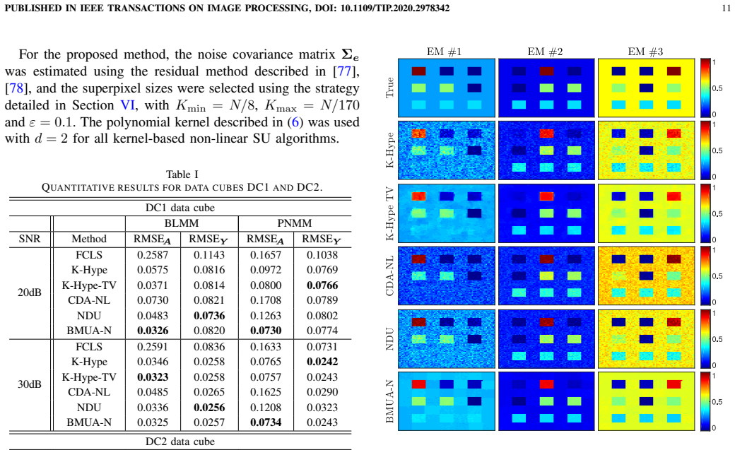
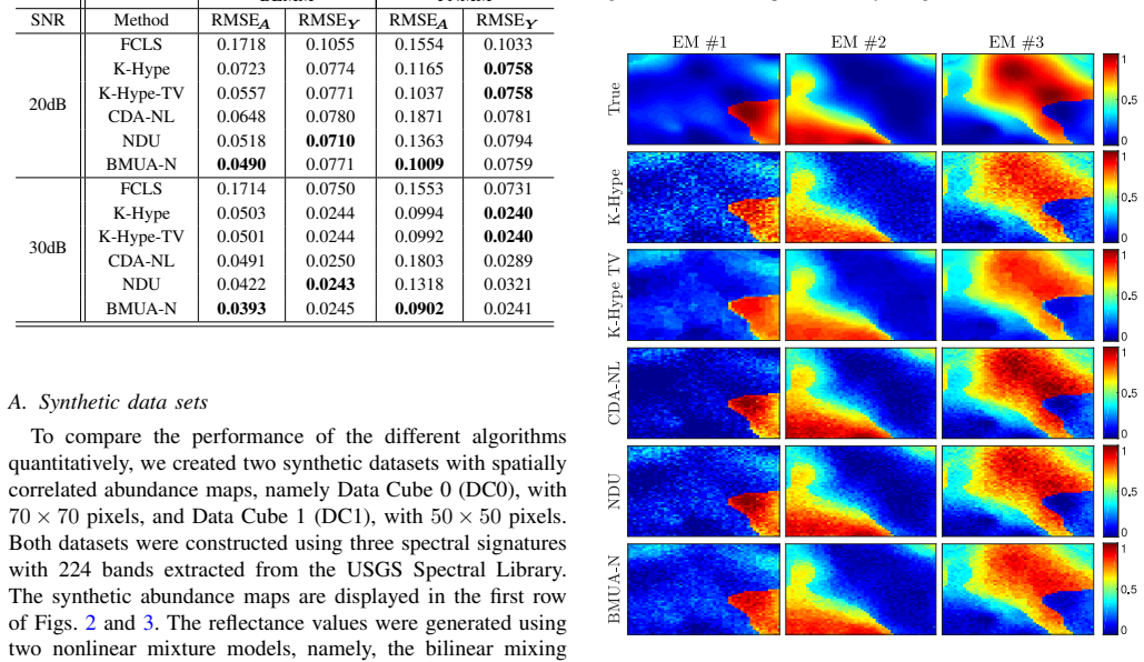
- [Section VIII-A] The text introduces the two synthetic datasets as DC0 and DC1, but Table I reports results for 'DC1' and 'DC2'. Please reconcile the naming of the synthetic cubes.
- [Table I] The quantitative comparisons report single-run RMSE values without standard deviations or repeated realizations; given that some margins are small (e.g., DC1 BLMM 30dB, RMSEA 0.0325 vs. 0.0323), a repeated-trial summary would strengthen the claim that BMUA-N outperforms the competing algorithms.
- [Section IV-C, Eq. (23)] The quantity yDn is used in Eq. (23) but never formally defined; please define it explicitly as the fine-domain image obtained by mapping the coarse image back to the original grid, consistent with the definition of âDn in (11).
- [References] References [21] and [35] appear to be the same paper (Chen, Richard and Honeine, IEEE TGRS 2014); please deduplicate and renumber accordingly.
Circularity Check
No significant circularity: the regularization constants are derived from noise statistics and explicit statistical assumptions, not fitted to the abundance outputs.
full rationale
The paper's derivation chain is self-contained. C0 and C1 follow from the noise-plus-modeling-error decomposition and assumptions A1-A5 (Eqs. 13-22); C2 is derived from the A6 uncorrelatedness identity (Eqs. 23-31), and the resulting expression is used as a constraint rather than as a fitted constant. The coarse-scale estimates âDn and ψ̂Cn enter the fine-scale problem as a regularizer, but this is a two-scale modeling choice, not a prediction of the fine-scale abundances from a parameter fitted to those same abundances. The strong-duality claim (Theorem 1) is proved in Appendix A using an external theorem [71], with the self-citation [72] only pointing to the supplemental material. The multiscale construction cites the authors' prior work [40], [41] for the general strategy, but the kernel-based statistical parameter derivation is new and does not depend on those citations as evidence. The manual setting of σ²_eψ in the experiments weakens the 'fully blind' claim but is a parameter choice, not a circular reduction. Assumptions A3 and A6 may be violated in practice, which would bias C0 or the Eq. (32) constraint, but that is a correctness/robustness concern, not circularity: no equation is equal to its own input by construction.
Assumptions & free parameters
free parameters (3)
- modeling error variance sigma^2_e,psi =
10^-8 * (1/N) * sum ||y_n||^2 in experiments
- superpixel search range and homogeneity tolerance (Kmin, Kmax, epsilon) =
N/8, N/170, 0.1
- polynomial kernel degree d and offset c =
d=2, c=1
assumptions (6)
- standard math RKHS representer theorem: optimal psi_n lies in the span of kernel evaluations at the endmember spectra
- standard math Strong duality criterion of Tuy and Tuan (Theorem 6 of [71]) applies to the quadratically constrained problems
- domain assumption Assumptions A1-A5: noise uncorrelated across pixels, modeling errors roughly constant within each superpixel, homogeneous noise covariance
- domain assumption Assumption A6: the three scale-difference vectors in equation (25) are mutually uncorrelated and zero-mean
- domain assumption Superpixel homogeneity can be measured by the ratio of the two largest singular values in equation (54)
- domain assumption Polynomial kernel of degree 2 captures the relevant nonlinear mixing
Cite this review
Pith. "Pith review of A Blind Multiscale Spatial Regularization Framework for Kernel-based Spectral Unmixing." pith.science (2026). https://pith.science/paper/FJUITKZ5
@misc{pith2026190806925,
  author       = {Pith},
  title        = {Pith review of: A Blind Multiscale Spatial Regularization Framework for Kernel-based Spectral Unmixing},
  year         = {2026},
  howpublished = {\url{https://pith.science/paper/FJUITKZ5}},
  note         = {Machine review of arXiv:1908.06925}
}
read the original abstract
Introducing spatial prior information in hyperspectral imaging (HSI) analysis has led to an overall improvement of the performance of many HSI methods applied for denoising, classification, and unmixing. Extending such methodologies to nonlinear settings is not always straightforward, specially for unmixing problems where the consideration of spatial relationships between neighboring pixels might comprise intricate interactions between their fractional abundances and nonlinear contributions. In this paper, we consider a multiscale regularization strategy for nonlinear spectral unmixing with kernels. The proposed methodology splits the unmixing problem into two sub-problems at two different spatial scales: a coarse scale containing low-dimensional structures, and the original fine scale. The coarse spatial domain is defined using superpixels that result from a multiscale transformation. Spectral unmixing is then formulated as the solution of quadratically constrained optimization problems, which are solved efficiently by exploring their strong duality and a reformulation of their dual cost functions in the form of root-finding problems. Furthermore, we employ a theory-based statistical framework to devise a consistent strategy to estimate all required parameters, including both the regularization parameters of the algorithm and the number of superpixels of the transformation, resulting in a truly blind (from the parameters setting perspective) unmixing method. Experimental results attest the superior performance of the proposed method when comparing with other, state-of-the-art, related strategies.
Figures

Figures from the paper (3 more)


Reference graph
Works this paper leans on
-
[1]
Hyperspectral remote sensing data analysis and future challenges,
J. M. Bioucas-Dias, A. Plaza, G. Camps-Valls, P. Scheunders, N. Nasrabadi, and J. Chanussot, “Hyperspectral remote sensing data analysis and future challenges,” IEEE Geoscience and Remote Sensing Magazine, vol. 1, no. 2, pp. 6–36, 2013
2013
-
[2]
Nonlinear unmixing of hyperspectral images: Models and algorithms,
N. Dobigeon, J.-Y . Tourneret, C. Richard, J. C. M. Bermudez, S. McLaughlin, and A. O. Hero, “Nonlinear unmixing of hyperspectral images: Models and algorithms,” IEEE Signal Processing Magazine , vol. 31, no. 1, pp. 82–94, Jan 2014
work page 2014
-
[3]
T. Imbiriba, J. C. M. Bermudez, C. Richard, and J.-Y . Tourneret, “Nonparametric detection of nonlinearly mixed pixels and endmember estimation in hyperspectral images,” IEEE Transactions on Image Pro- cessing, vol. 25, no. 3, pp. 1136–1151, March 2016
work page 2016
-
[4]
Endmember variability in spectral mixture analysis: A review,
B. Somers, G. P. Asner, L. Tits, and P. Coppin, “Endmember variability in spectral mixture analysis: A review,” Remote Sensing of Environment, vol. 115, no. 7, pp. 1603–1616, 2011
work page 2011
-
[5]
Generalized linear mixing model accounting for endmember variability,
T. Imbiriba, R. A. Borsoi, and J. C. M. Bermudez, “Generalized linear mixing model accounting for endmember variability,” in 2018 IEEE International Conference on Acoustics, Speech and Signal Processing (ICASSP). Calgary, Canada: IEEE, 2018, pp. 1862–1866
work page 2018
-
[6]
R. A. Borsoi, T. Imbiriba, and J. C. M. Bermudez, “Super-resolution for hyperspectral and multispectral image fusion accounting for seasonal spectral variability,” IEEE Transactions on Image Processing , vol. 29, pp. 116–127, 2020
work page 2020
-
[7]
Deep generative endmember modeling: An application to un- supervised spectral unmixing,
——, “Deep generative endmember modeling: An application to un- supervised spectral unmixing,” IEEE Transactions on Computational Imaging, vol. 6, pp. 374–384, 2020
work page 2020
-
[8]
Deep generative models for library augmentation in multiple endmember spectral mixture analysis,
R. A. Borsoi, T. Imbiriba, J. C. M. Bermudez, and C. Richard, “Deep generative models for library augmentation in multiple endmember spectral mixture analysis,” arXiv preprint, 2019
work page 2019
Show all 79 references
-
[10]
Nonlinear spectral mixing in desert vegetation,
T. W. Ray and B. C. Murray, “Nonlinear spectral mixing in desert vegetation,” Remote Sensing of Environment , vol. 55, no. 1, pp. 59–64, 1996
1996
-
[11]
A review of nonlinear hyperspec- tral unmixing methods,
R. Heylen, M. Parente, and P. Gader, “A review of nonlinear hyperspec- tral unmixing methods,” IEEE Journal of Selected Topics in Applied Earth Observations and Remote Sensing , vol. 7, no. 6, pp. 1844–1868, June 2014
2014
-
[12]
Photometric phase functions of common geologic minerals and applications to quantitative analysis of mineral mixture reflectance spectra,
J. F. Mustard and C. M. Pieters, “Photometric phase functions of common geologic minerals and applications to quantitative analysis of mineral mixture reflectance spectra,” Journal of Geophysical Research: Solid Earth, vol. 94, no. B10, pp. 13 619–13 634, 1989
1989
-
[13]
A quantitative and comparative analysis of linear and nonlinear spectral mixture models using radial basis function neural networks,
K. J. Guilfoyle, M. L. Althouse, and C.-I. Chang, “A quantitative and comparative analysis of linear and nonlinear spectral mixture models using radial basis function neural networks,” IEEE Transactions on Geoscience and Remote Sensing , vol. 39, no. 10, pp. 2314–2318, 2001
2001
-
[14]
Supervised nonlinear spectral unmixing using a postnonlinear mixing model for hy- perspectral imagery,
Y . Altmann, A. Halimi, N. Dobigeon, and J. Y . Tourneret, “Supervised nonlinear spectral unmixing using a postnonlinear mixing model for hy- perspectral imagery,” IEEE Transactions on Image Processing , vol. 21, no. 6, pp. 3017–3025, June 2012
2012
-
[15]
Abundance estimation from hyperspec- tral image based on probabilistic outputs of multi-class support vector machines,
P.-X. Li, B. Wu, and L. Zhang, “Abundance estimation from hyperspec- tral image based on probabilistic outputs of multi-class support vector machines,” in 2005 IEEE International Geoscience and Remote Sensing Symposium (IGARSS), vol. 6, July 2005, pp. 4315–4318
2005
-
[16]
Non-linear spectral unmixing by geodesic simplex volume maximization,
R. Heylen, D. Burazerovic, and P. Scheunders, “Non-linear spectral unmixing by geodesic simplex volume maximization,” IEEE Journal of Selected Topics in Signal Processing , vol. 5, no. 3, pp. 534–542, 2011
2011
-
[17]
A distance geometric framework for nonlinear hyperspectral unmixing,
R. Heylen and P. Scheunders, “A distance geometric framework for nonlinear hyperspectral unmixing,” IEEE Journal of Selected Topics in Applied Earth Observations and Remote Sensing, vol. 7, no. 6, pp. 1879– 1888, June 2014
2014
-
[18]
A kernel spatial complexity-based nonlinear unmixing method of hyperspectral imagery,
X. Wu, X. Li, and L. Zhao, “A kernel spatial complexity-based nonlinear unmixing method of hyperspectral imagery,” in Proc. LSMS/ICSEE , 2010, pp. 451–458
2010
-
[19]
Blind nonlinear hyperspectral unmixing based on constrained kernel nonnegative matrix factorization,
X. Li, J. Cui, and L. Zhao, “Blind nonlinear hyperspectral unmixing based on constrained kernel nonnegative matrix factorization,” Signal, Image and Video Processing , vol. 8, no. 8, pp. 1555–1567, 2012
2012
-
[20]
Nonlinear unmixing of hyperspec- tral data based on a linear-mixture/nonlinear-fluctuation model,
J. Chen, C. Richard, and P. Honeine, “Nonlinear unmixing of hyperspec- tral data based on a linear-mixture/nonlinear-fluctuation model,” IEEE Transactions on Signal Processing , vol. 61, pp. 480–492, Jan 2013
2013
-
[21]
Nonlinear estimation of material abundances in hyperspectral images with 𝓁1-norm spatial regularization,
——, “Nonlinear estimation of material abundances in hyperspectral images with 𝓁1-norm spatial regularization,” IEEE Transactions on Geoscience and Remote Sensing , vol. 52, no. 5, pp. 2654–2665, May 2014
2014
-
[22]
Nonlin- ear spectral unmixing of hyperspectral images using gaussian processes,
Y . Altmann, N. Dobigeon, S. McLaughlin, and J.-Y . Tourneret, “Nonlin- ear spectral unmixing of hyperspectral images using gaussian processes,” IEEE Transactions on Signal Processing , vol. 61, pp. 2442–2453, May 2013
2013
-
[23]
Nonlinear unmixing of hyperspectral data with vector-valued kernel functions,
R. Ammanouil, A. Ferrari, C. Richard, and S. Mathieu, “Nonlinear unmixing of hyperspectral data with vector-valued kernel functions,” IEEE Transactions on Image Processing , vol. 26, no. 1, pp. 340–354, 2017
2017
-
[24]
Incorporating spatial information in spectral unmixing: A review,
C. Shi and L. Wang, “Incorporating spatial information in spectral unmixing: A review,” Remote Sensing of Environment , vol. 149, pp. 70–87, 2014
2014
-
[25]
A low-rank tensor regularization strategy for hyperspectral unmixing,
T. Imbiriba, R. A. Borsoi, and J. C. M. Bermudez, “A low-rank tensor regularization strategy for hyperspectral unmixing,” in 2018 IEEE Statistical Signal Processing Workshop (SSP) , 2018, pp. 373–377
2018
-
[26]
Total variation spatial regularization for sparse hyperspectral unmixing,
M.-D. Iordache, J. M. Bioucas-Dias, and A. Plaza, “Total variation spatial regularization for sparse hyperspectral unmixing,” IEEE Transac- tions on Geoscience and Remote Sensing, vol. 50, no. 11, pp. 4484–4502, 2012
2012
-
[27]
Adaptive spatial regularization sparse unmixing strategy based on joint MAP for hyperspectral remote sensing imagery,
R. Feng, Y . Zhong, and L. Zhang, “Adaptive spatial regularization sparse unmixing strategy based on joint MAP for hyperspectral remote sensing imagery,” IEEE Journal of Selected Topics in Applied Earth Observations and Remote Sensing , vol. 9, no. 12, pp. 5791–5805, 2016
2016
-
[28]
Blind hyperspectral unmixing using an extended linear mixing model to address spectral variability,
L. Drumetz, M.-A. Veganzones, S. Henrot, R. Phlypo, J. Chanussot, and C. Jutten, “Blind hyperspectral unmixing using an extended linear mixing model to address spectral variability,” IEEE Transactions on Image Processing, vol. 25, no. 8, pp. 3890–3905, 2016
2016
-
[29]
Low-rank tensor modeling for hyperspectral unmixing accounting for spectral variability,
T. Imbiriba, R. A. Borsoi, and J. C. M. Bermudez, “Low-rank tensor modeling for hyperspectral unmixing accounting for spectral variability,” IEEE Transactions on Geoscience and Remote Sensing , vol. 58, no. 3, pp. 1833–1842, March 2020
2020
-
[30]
Improved hyperspectral unmixing with endmember variability parametrized using an interpolated scaling tensor,
R. A. Borsoi, T. Imbiriba, and J. C. Moreira Bermudez, “Improved hyperspectral unmixing with endmember variability parametrized using an interpolated scaling tensor,” in 2019 IEEE International Conference on Acoustics, Speech and Signal Processing (ICASSP) , May 2019, pp. 2177–2181
2019
-
[31]
An augmented linear mixing model to address spectral variability for hyperspectral unmixing,
D. Hong, N. Yokoya, J. Chanussot, and X. X. Zhu, “An augmented linear mixing model to address spectral variability for hyperspectral unmixing,” IEEE Transactions on Image Processing, vol. 28, no. 4, pp. 1923–1938, 2019
1923
-
[32]
Sulora: Subspace unmixing with low-rank attribute embedding for hyperspectral data analysis,
D. Hong and X. X. Zhu, “Sulora: Subspace unmixing with low-rank attribute embedding for hyperspectral data analysis,” IEEE Journal of Selected Topics in Signal Processing , vol. 12, no. 6, pp. 1351–1363, 2018
2018
-
[33]
Relationships between nonlinear and space-variant linear models in hyperspectral image unmixing,
L. Drumetz, B. Ehsandoust, J. Chanussot, B. Rivet, M. Babaie-Zadeh, and C. Jutten, “Relationships between nonlinear and space-variant linear models in hyperspectral image unmixing,” IEEE Signal Processing Letters, vol. 24, no. 10, pp. 1567–1571, 2017
2017
-
[34]
Integrating spatial information in the normalized p-linear algorithm for nonlinear hyperspectral unmixing,
M. Tang, L. Gao, A. Marinoni, P. Gamba, and B. Zhang, “Integrating spatial information in the normalized p-linear algorithm for nonlinear hyperspectral unmixing,” IEEE Journal of Selected Topics in Applied Earth Observations and Remote Sensing , vol. 11, no. 4, pp. 1179–1190, 2018
2018
-
[35]
Nonlinear estimation of material abundances in hyperspectral images with L1-norm spatial regulariza- tion,
J. Chen, C. Richard, and P. Honeine, “Nonlinear estimation of material abundances in hyperspectral images with L1-norm spatial regulariza- tion,” Geoscience and Remote Sensing, IEEE Transactions on , vol. 52, no. 5, pp. 2654–2665, 2014
2014
-
[36]
Centralized collaborative sparse unmixing for hyperspectral images,
R. Wang, H.-C. Li, W. Liao, X. Huang, and W. Philips, “Centralized collaborative sparse unmixing for hyperspectral images,” IEEE Journal of Selected Topics in Applied Earth Observations and Remote Sensing , vol. 10, no. 5, pp. 1949–1962, 2017
1949
-
[37]
Nonconvex-sparsity and nonlocal-smoothness-based blind hyperspectral unmixing,
J. Yao, D. Meng, Q. Zhao, W. Cao, and Z. Xu, “Nonconvex-sparsity and nonlocal-smoothness-based blind hyperspectral unmixing,” IEEE Transactions on Image Processing, vol. 28, no. 6, pp. 2991–3006, 2019
2019
-
[38]
Manifold regularized sparse NMF for hyperspectral unmixing,
X. Lu, H. Wu, Y . Yuan, P. Yan, and X. Li, “Manifold regularized sparse NMF for hyperspectral unmixing,” IEEE Transactions on Geoscience and Remote Sensing , vol. 51, no. 5, pp. 2815–2826, 2012
2012
-
[39]
A graph laplacian regular- ization for hyperspectral data unmixing,
R. Ammanouil, A. Ferrari, and C. Richard, “A graph laplacian regular- ization for hyperspectral data unmixing,” in 2015 IEEE International Conference on Acoustics, Speech and Signal Processing (ICASSP) . IEEE, 2015, pp. 1637–1641
2015
-
[40]
A fast multiscale spatial regularization for sparse hyperspectral unmixing,
R. A. Borsoi, T. Imbiriba, J. C. M. Bermudez, and C. Richard, “A fast multiscale spatial regularization for sparse hyperspectral unmixing,” IEEE Geoscience and Remote Sensing Letters , vol. 16, no. 4, pp. 598– 602, April 2019
2019
-
[41]
A data dependent multiscale model for hyperspectral unmixing with spectral variability,
R. A. Borsoi, T. Imbiriba, and J. C. M. Bermudez, “A data dependent multiscale model for hyperspectral unmixing with spectral variability,” IEEE Transactions on Image Processing, vol. 29, pp. 3638–3651, 2020
2020
-
[42]
Regularization pa- rameter estimation for non-negative hyperspectral image deconvolution,
Y . Song, D. Brie, E.-H. Djermoune, and S. Henrot, “Regularization pa- rameter estimation for non-negative hyperspectral image deconvolution,” IEEE Transactions on Image Processing, vol. 25, no. 11, pp. 5316–5330, 2016
2016
-
[43]
Functions of positive and negative type and their connection with the theory of integral equations,
J. Mercer, “Functions of positive and negative type and their connection with the theory of integral equations,” Philos. Trans. Roy. Soc. London Ser. A, vol. 209, pp. 415–446, 1909
1909
-
[44]
On properly positive hermitian matrices,
E. H. Moore, “On properly positive hermitian matrices,” Bull. American Mathematical Society, vol. 23, p. 59, 1916
1916
-
[45]
Theory of reproducing kernels,
N. Aronszajn, “Theory of reproducing kernels,” Transactions of the American Mathematical Society , vol. 68, 1950
1950
-
[46]
Kreyszig, Introductory functional analysis with applications
E. Kreyszig, Introductory functional analysis with applications . Wiley New York, 1989, vol. 81
1989
-
[47]
Steinwart and A
I. Steinwart and A. Christmann, Support vector machines . Springer, 2008
2008
-
[48]
V . N. Vapnik, The nature of statistical learning theory . New York, NY: Springer, 1995
1995
-
[49]
Schölkopf and A
B. Schölkopf and A. J. Smola, Learning with Kernels: Support Vector Machines, Regularization, Optimization, and Beyond . The MIT Press, 2001
2001
-
[50]
C. E. Rasmussen and C. K. I. Williams, Gaussian Processes for Machine Learning. The MIT Press, 2006
2006
-
[51]
Nonlinear hyperspectral mixture analysis for tree cover estimates in orchards,
B. Somers, K. Cools, S. Delalieux, J. Stuckens, D. V . der Zande, W. W. Verstraeten, and P. Coppin, “Nonlinear hyperspectral mixture analysis for tree cover estimates in orchards,” Remote Sensing of Environment , vol. 113, no. 6, pp. 1183–1193, February 2009
2009
-
[52]
J. A. K. Suykens, T. V . Gestel, J. D. Brabanter, B. D. Moor, and J. Vandewalle, Least Squares Support Vector Machines . Singapore: World Scientific, 2002
2002
-
[54]
Spectral-density- based graph construction techniques for hyperspectral image analysis,
J. R. Stevens, R. G. Resmini, and D. W. Messinger, “Spectral-density- based graph construction techniques for hyperspectral image analysis,” IEEE Transactions on Geoscience and Remote Sensing , vol. 55, no. 10, pp. 5966–5983, 2017
2017
-
[55]
SLIC superpixels compared to state-of-the-art superpixel methods,
R. Achanta, A. Shaji, K. Smith, A. Lucchi, P. Fua, and S. Süsstrunk, “SLIC superpixels compared to state-of-the-art superpixel methods,” IEEE Transactions on Pattern Analysis and Machine Intelligence , vol. 34, no. 11, pp. 2274–2282, 2012
2012
-
[56]
Boundary extraction in natural images using ultrametric contour maps,
P. Arbelaez, “Boundary extraction in natural images using ultrametric contour maps,” in 2006 Conference on Computer Vision and Pattern Recognition Workshop (CVPRW’06). IEEE, 2006, pp. 182–182
2006
-
[57]
Hyperspectral image segmentation using a new spectral unmixing-based binary partition tree representation,
M. A. Veganzones, G. Tochon, M. Dalla-Mura, A. J. Plaza, and J. Chanussot, “Hyperspectral image segmentation using a new spectral unmixing-based binary partition tree representation,” IEEE Transactions on Image Processing , vol. 23, no. 8, pp. 3574–3589, 2014
2014
-
[58]
Spatial group sparsity reg- ularized nonnegative matrix factorization for hyperspectral unmixing,
X. Wang, Y . Zhong, L. Zhang, and Y . Xu, “Spatial group sparsity reg- ularized nonnegative matrix factorization for hyperspectral unmixing,” IEEE Transactions on Geoscience and Remote Sensing , vol. 55, no. 11, pp. 6287–6304, 2017
2017
-
[59]
Generalized cross-validation as a method for choosing a good ridge parameter,
G. H. Golub, M. Heath, and G. Wahba, “Generalized cross-validation as a method for choosing a good ridge parameter,” Technometrics, vol. 21, no. 2, pp. 215–223, 1979
1979
-
[60]
Stein Unbiased GrA- dient estimator of the Risk (SUGAR) for multiple parameter selection,
C.-A. Deledalle, S. Vaiter, J. Fadili, and G. Peyré, “Stein Unbiased GrA- dient estimator of the Risk (SUGAR) for multiple parameter selection,” SIAM Journal on Imaging Sciences , vol. 7, no. 4, pp. 2448–2487, 2014
2014
-
[61]
ADA-PT: An adaptive parameter tuning strategy based on the weighted stein unbiased risk estimator,
R. Ammanouil, A. Ferrari, and C. Richard, “ADA-PT: An adaptive parameter tuning strategy based on the weighted stein unbiased risk estimator,” in 2018 IEEE International Conference on Acoustics, Speech and Signal Processing (ICASSP) . IEEE, 2018, pp. 4449–4453
2018
-
[62]
Efficient determination of multiple regularization parameters in a generalized L-curve framework,
M. Belge, M. E. Kilmer, and E. L. Miller, “Efficient determination of multiple regularization parameters in a generalized L-curve framework,” Inverse Problems, vol. 18, no. 4, pp. 1161–1183, 2002
2002
-
[63]
Common structure of techniques for choosing smoothing parameters in regression problems,
P. Hall and D. M. Titterington, “Common structure of techniques for choosing smoothing parameters in regression problems,” Journal of the Royal Statistical Society: Series B (Methodological) , vol. 49, no. 2, pp. 184–198, 1987
1987
-
[64]
A study of methods of choosing the smoothing parameter in image restoration by regularization,
A. M. Thompson, J. C. Brown, J. W. Kay, and D. M. Titterington, “A study of methods of choosing the smoothing parameter in image restoration by regularization,” IEEE Transactions on Pattern Analysis & Machine Intelligence, no. 4, pp. 326–339, 1991
1991
-
[65]
Methods for choosing the regularization parameter and estimating the noise variance in image restoration and their relation,
N. P. Galatsanos and A. K. Katsaggelos, “Methods for choosing the regularization parameter and estimating the noise variance in image restoration and their relation,” IEEE Transactions on image processing , vol. 1, no. 3, pp. 322–336, 1992
1992
-
[66]
A. N. Heinz Werner Engl, Martin Hanke, Regularization of Inverse Problems (Mathematics and Its Applications) , 1st ed., ser. Mathematics and Its Applications. Springer, 1996
1996
-
[67]
The application of constrained least squares estimation to image restoration by digital computer,
B. R. Hunt, “The application of constrained least squares estimation to image restoration by digital computer,” IEEE Transactions on Comput- ers, vol. 100, no. 9, pp. 805–812, 1973
1973
-
[68]
Bayesian nonlinear hyperspectral unmixing with spatial residual component analysis,
Y . Altmann, M. Pereyra, and S. McLaughlin, “Bayesian nonlinear hyperspectral unmixing with spatial residual component analysis,” IEEE Transactions on Computational Imaging , vol. 1, no. 3, pp. 174–185, 2015
2015
-
[69]
Spatial regularization for nonlinear unmixing of hyperspectral data with vector- valued kernel functions,
R. Ammanouil, A. Ferrari, C. Richard, and J.-Y . Tournere, “Spatial regularization for nonlinear unmixing of hyperspectral data with vector- valued kernel functions,” in 2016 IEEE Statistical Signal Processing Workshop (SSP). IEEE, 2016, pp. 1–5
2016
-
[70]
Boyd and L
S. Boyd and L. Vandenberghe, Convex optimization . Cambridge university press, 2004
2004
-
[71]
Generalized S-lemma and strong duality in nonconvex quadratic programming,
H. Tuy and H. D. Tuan, “Generalized S-lemma and strong duality in nonconvex quadratic programming,” Journal of Global Optimization , vol. 56, no. 3, pp. 1045–1072, 2013
2013
-
[72]
A blind multiscale spatial regularization framework for kernel-based spectral unmixing,
R. A. Borsoi, T. Imbiriba, J. C. M. Bermudez, and C. Richard, “A blind multiscale spatial regularization framework for kernel-based spectral unmixing,” arXiv preprint arXiv:1908.06925 , 2019
1908 arXiv
-
[73]
The multivariate bisection algorithm,
M. L. Galván, “The multivariate bisection algorithm,” Revista de la Unión Matemática Argentina , pp. 79–98, Mar. 2019
2019
-
[74]
Bisection method in higher dimensions and the efficiency number,
D. Bachrathy and G. Stépán, “Bisection method in higher dimensions and the efficiency number,” Periodica Polytechnica Mechanical Engi- neering, vol. 56, no. 2, pp. 81–86, 2012
2012
-
[75]
Low-dimensional enhanced superpixel representation with homogeneity testing for unmixing of hyperspectral imagery,
J. Yi and M. Velez-Reyes, “Low-dimensional enhanced superpixel representation with homogeneity testing for unmixing of hyperspectral imagery,” in Algorithms and Technologies for Multispectral, Hyperspec- tral, and Ultraspectral Imagery XXIV, vol. 10644. International Society f...
2018
-
[76]
Hyperspectral unmixing in presence of endmember variability, nonlinearity, or mismodeling effects,
A. Halimi, P. Honeine, and J. M. Bioucas-Dias, “Hyperspectral unmixing in presence of endmember variability, nonlinearity, or mismodeling effects,” IEEE Transactions on Image Processing , vol. 25, no. 10, pp. 4565–4579, 2016
2016
-
[77]
Principal components transform with simple, automatic noise adjustment,
R. E. Roger, “Principal components transform with simple, automatic noise adjustment,” International Journal of Remote Sensing , vol. 17, no. 14, pp. 2719–2727, 1996
1996
-
[78]
Modified residual method for the estimation of noise in hyperspectral images
A. Mahmood, A. Robin, and M. Sears, “Modified residual method for the estimation of noise in hyperspectral images.” IEEE Transactions on Geoscience and Remote Sensing , vol. 55, no. 3, pp. 1451–1460, 2017
2017
-
[79]
Vertex Component Anal- ysis: A fast algorithm to unmix hyperspectral data,
J. M. P. Nascimento and J. M. Bioucas-Dias, “Vertex Component Anal- ysis: A fast algorithm to unmix hyperspectral data,” IEEE Transactions on Geoscience and Remote Sensing , vol. 43, no. 4, pp. 898–910, April 2005
2005
-
[80]
Strong duality for the CDT subproblem: a necessary and sufficient condition,
W. Ai and S. Zhang, “Strong duality for the CDT subproblem: a necessary and sufficient condition,” SIAM Journal on Optimization , vol. 19, no. 4, pp. 1735–1756, 2009
2009
-
[81]
Copositive relaxation beats Lagrangian dual bounds in quadratically and linearly constrained quadratic optimization problems,
I. M. Bomze, “Copositive relaxation beats Lagrangian dual bounds in quadratically and linearly constrained quadratic optimization problems,” SIAM Journal on Optimization , vol. 25, no. 3, pp. 1249–1275, 2015. Ricardo Augusto Borsoi (S’18) received the MSc degree in electrical ...
2015
Reviewed August 14, 2026 · model on record in the stance chip above.
Discussion (0). Continue with ORCID to comment.