REVIEW 3 major objections 7 minor 1 cited by
Matrix Inversion by Quantum Walk
T0 review · 3 major / 7 minor · reviewed 2026-08-05 · deepseek-v4-flash
Pith's one-line read The paper claims that matrix inversion reduces to a weakly coupled quantum walk, with no phase estimation, replacing HHL's central subroutine.
desk verdict Genuinely new simplification of HHL, but the central perturbative formula is wrong as stated; the result likely survives, but the proof needs a real fix. read the letter →
The pith
A machine-rendered reading of the paper's core claim, the machinery that carries it, and where it could break.
The reading
What carries the argument
The load-bearing object is the block-tridiagonal weak-coupling ladder: a chain of auxiliary sites coupled by strength $\gamma$, with the matrix $A$ bridging the two halves. In the singular-value basis each singular mode decouples into a small tridiagonal block, so the full evolution is a direct sum of finite-dimensional evolutions. Degenerate perturbation theory on the near-zero-energy sector makes the effective Hamiltonian proportional to $A^{-1}$; the high-energy eigenstates are the leading error, and lengthening the ladder suppresses their overlap with the input state.
What would settle it
For a single block with $\lambda=1$, $\gamma=0.1$, $t=10$, diagonalize the $2\times2$ block and compute $\alpha_n$ exactly; the exact value is about $0.104$ while Eq. (3) gives about $0.0948$, an 8% discrepancy. Repeating at smaller $\gamma$ (e.g. $0.01$) would show whether the discrepancy shrinks as $O(\gamma)$ — a slow but correct series — or persists, which would mean Eq. (3) mis-states the eigenvalues.
Extended reading notes
Core claim
The central claim is that matrix inversion is encoded in the low-energy sector of a tuned Hamiltonian. In the singular-value decomposition of $A$, the Hamiltonian $H$ with off-diagonal couplings $\gamma$ decomposes into $4\times4$ blocks $h_n = h_n^+\oplus h_n^-$, spanned by the states $|n_{1\pm}\rangle,|n_{2\pm}\rangle$. Up to normalization, the transition amplitude from the input block to the output block is $\alpha_n = \tfrac12(\langle n_1^+|e^{-ih_n t}|n_1^+\rangle - \langle n_1^-|e^{-ih_n t}|n_1^-\rangle)$, and the paper derives $\alpha_n \propto \gamma/\lambda_n + O(\gamma^2\kappa^2)$. Thus post-selected evolution yields $|\psi\rangle = \sum_n \langle\eta_n|b\rangle\alpha_n|\lambda_n\r
Load-bearing premise
The derivation assumes the perturbative expansion of the transition amplitude $\alpha_n$ in powers of $x=\gamma/\lambda_n$, specifically Eq. (3), is correct; if that formula does not reproduce the exact $2\times2$-block evolution at the chosen $\gamma$, the $O(\gamma\kappa^2)$ error bound is not established.
Editorial extensions
If this is right
- Matrix inversion becomes one Hamiltonian evolution plus post-selection, with no phase estimation; the simplest version matches the $O(\kappa^2)$ condition-number scaling of HHL.
- With one additional weakly coupled site, the error improves to $O(\gamma^3\kappa^3)$; choosing $\gamma=\delta/\kappa^{3/2}$ gives runtime $O(\kappa^{3/2}T/\delta)$.
- Longer ladders plus a linear combination of unitaries cancel errors to arbitrary order with $R\sim\log(1/\varepsilon)$, recovering the best known precision dependence.
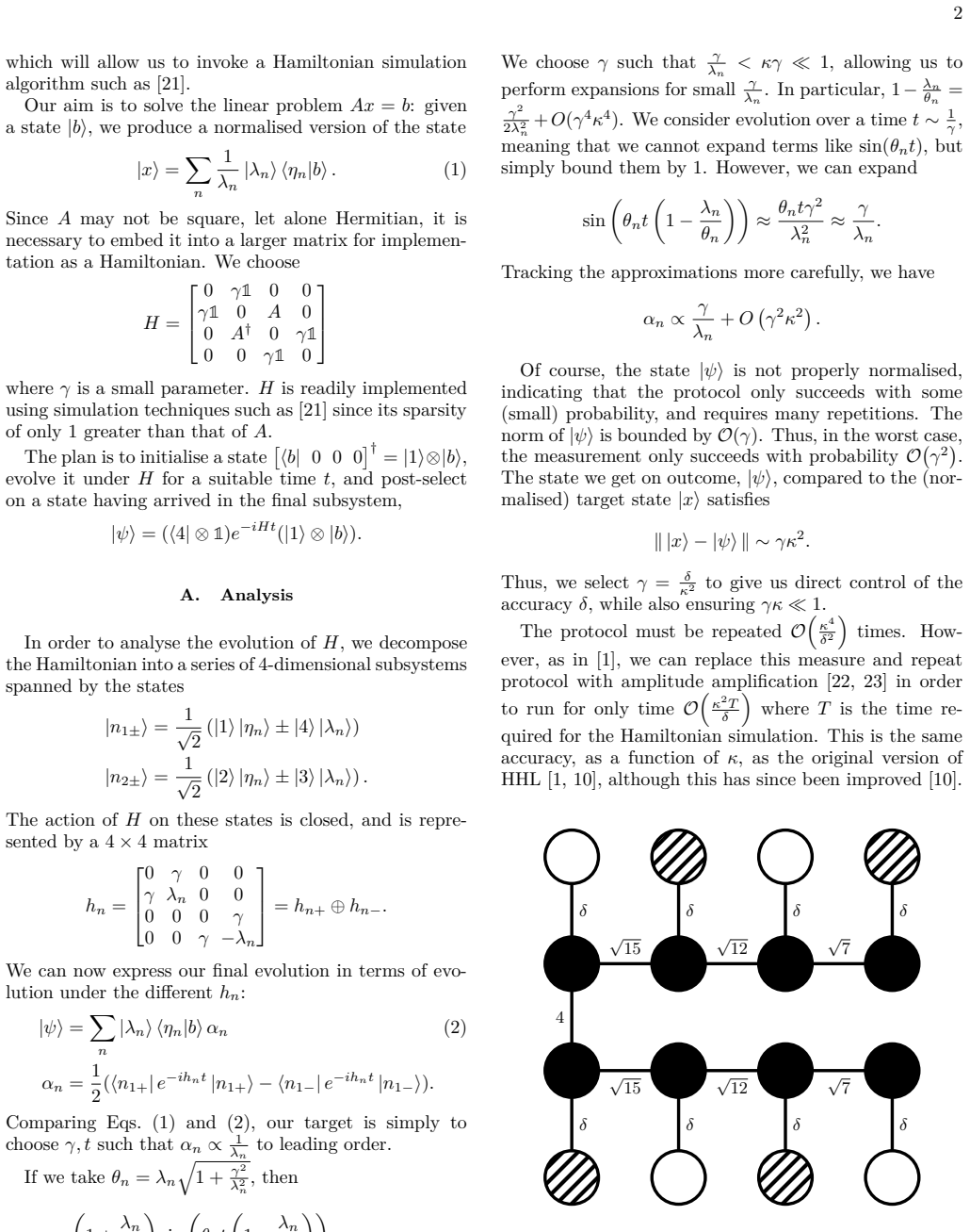
- The four-qubit example ($\kappa=1$, $\delta=0.01$) achieves the predicted $O(\delta)$ accuracy, and the coupling graph maps onto spin-exchange, photonic, or superconducting chains.
- The protocol succeeds with probability $O(\gamma^2)$ before amplitude amplification; repeat-until-success is a viable small-device alternative.
Reading between the lines
- Beyond inversion, the same weak-coupling construction is a plausible template for preparing $f(A)|b\rangle$ for other spectral functions, since the perturbation expansion already realizes $A^{-1}$ as an effective Hamiltonian.
- Because no eigenvalue is ever measured, the method could run on analog or Hamiltonian-based devices where a fixed engineered interaction replaces a gate-by-gate phase-estimation circuit.
- The small success probability means the advertised runtime depends heavily on amplitude amplification; at small scale, the repeat-until-success overhead may dominate.
- The quickest independent check is numerical: comparing exact block amplitudes with Eq. (3) at a few values of $\gamma$ decides whether the perturbative core is sound before hardware effort is invested.
Editorial analysis
A structured set of objections, weighed in public.
Referee Report
Summary. The paper presents a quantum algorithm for matrix inversion that replaces the phase-estimation stages of HHL with a continuous-time quantum walk. The matrix A is embedded into a larger Hamiltonian H, with a weak coupling γ; evolving for time t and post-selecting on a final register gives a state whose amplitudes are, to leading order, γ/λ_n, i.e. proportional to A^{-1}|b⟩. Section I derives the basic version and claims error O(γκ²), with the same κ scaling as original HHL. Section II extends H with additional couplings to suppress high-energy leakage, giving improved accuracy and, via a conjectured construction, near-optimal scaling. Three worked examples are given, along with a table of numerically determined coupling strengths for R≤6. The core analytic formula, Eq. (3), is, however, not the correct transition amplitude for the stated 2×2 blocks, so the proof of the central error bound is not sound as written.
Significance. The algorithmic idea is potentially significant: if the perturbation analysis can be repaired, the protocol offers a conceptually simpler route to matrix inversion, using Hamiltonian simulation plus post-selection/amplitude amplification and no phase estimation. The construction is not circular: the constants γ and J_n are chosen to satisfy algebraic conditions, and the numerical examples appear to confirm the predicted leading-order behavior. However, the paper's main theoretical claim currently rests on an incorrect analytical formula. The extension to the best known condition-number/precision scaling depends on an unproven conjecture with only numerical evidence for small R. With a corrected derivation the result would be a useful simplification of HHL; as it stands, the proof needs substantial revision.
major comments (3)
- [Section I, Eq. (3)] Eq. (3) is not the correct transition amplitude for the stated Hamiltonian blocks. For h_{n+} = [[0,γ],[γ,λ_n]], the (1,1) survival amplitude is A_+ = [E_+ e^{-iE_- t} - E_- e^{-iE_+ t}]/Ω with Ω=√(λ_n²+4γ²), E_±=(λ_n±Ω)/2; for h_{n-} the corresponding amplitude is A_- = [E_+ e^{iE_- t} - E_- e^{iE_+ t}]/Ω. Hence α_n = (A_+ - A_-)/2 = (i/Ω)[E_- sin(E_+ t) - E_+ sin(E_- t)]. This differs from Eq. (3) in the energy denominator (√(λ_n²+γ²) vs.√(λ_n²+4γ²)) and in the phase structure. A numerical check at λ=1, γ=0.1, t=10 gives |α_n|≈0.104, while Eq. (3) gives ≈0.0948. Since the paper's central claim α_n ∝ γ/λ_n + O(γ²κ²), and hence the O(γκ²) error bound, is obtained by expanding Eq. (3), that derivation is not valid as written. The authors must replace Eq. (3) with the exact expression and redo the perturbative expansion, including a uniform bound over singular values in [1/κ,1].
- [Section I, error bound] The statement after Eq. (3) that ∥|x⟩−|ψ⟩∥∼γκ² needs a rigorous derivation. The state |ψ⟩ defined in Eq. (2) is unnormalized, so the comparison with the normalized target |x⟩ must be made after normalization. In addition, the correction term O(γ²κ²) in α_n must be uniform in n, and the bound must account for the coherent sum over n in Eq. (2). This is not a cosmetic point: the choice γ=δ/κ² and the claimed run-time O(κ²T/δ) depend on this eps/delta relation. Please state and prove the uniform error bound carefully.
- [Section II, Conjecture 1 and Conclusion] The Conclusion states that the protocol has 'matched the best performance [10,11]' in terms of accuracy and condition number. This asymptotic claim is conditional on Conjecture 1, for which the paper provides numerical solutions only up to R=6 and explicitly acknowledges that existence is unknown. The conclusion should be phrased conditionally. In addition, Lemma 1's proof is hard to follow: the equation \tilde h |λ_L⟩ + |R⟩ = λ |λ_L⟩ omits the factors γ and J_R that appear in h_+, and the subsequent bound is not fully specified in terms of the original Hamiltonian parameters. Please clarify the scaling and the exact eigenvalue equation, since this lemma is load-bearing for the high-order suppression claim.
minor comments (7)
- [Section I] The text 'γ/λ_n < κγ≪1' is strange; the first inequality is equivalent to 1/λ_n < κ, which is already true by the conditioning assumption. The intended condition is presumably γκ≪1.
- [Section I] In the displayed Hamiltonian, 'γ1' and 'A 0' should use explicit identity matrices, e.g. γ I, to avoid confusion with the scalar γ.
- [Eq. (3)] Eq. (3) uses a proportionality sign ∝ but gives an explicit formula with no proportionality factor; if an overall n-independent constant is intended, it should be stated.
- [Example 3] The text says α_n = 0.869923 i γ/λ + O(γ⁶/λ⁶), but then concludes with O(γ⁵κ⁶). The exponents should be reconciled.
- [Abstract / Conclusion] The abstract says the approach 'relies solely on Hamiltonian simulation', but the protocol also uses post-selection and, in the improved version, amplitude amplification. Please rephrase to avoid overstatement.
- [Conclusion] Typo: 'far more direct that HHL' should be 'far more direct than HHL'.
- [Appendix A / Table I] The role of the fixed evolution time t=2π/γ and the footnote about renormalizing \tilde h should be brought into the main text, since they affect the quoted run time.
Circularity Check
No significant circularity: the algorithm is a constructive design whose output follows from an explicit perturbative expansion, with no load-bearing self-citations or fitted predictions.
full rationale
The paper's derivation chain is self-contained. The Hamiltonian H is defined by embedding A with a weak coupling γ, and the post-selected amplitude α_n is computed from the exact Schrödinger evolution in a reduced subspace (Eq. 2). The central claim α_n ∝ γ/λ_n is obtained by expanding the explicit expression in Eq. (3) in powers of γ/λ_n, not by assuming the target output. The parameters γ and the coupling strengths J_n in Table I are solutions of algebraic design equations derived from the same expansion; they are not fitted to simulation data or to the desired output state. The only self-citations are auxiliary: [24] provides code examples for the numerical illustrations and [25] is a review of perfect state transfer used for an implementation mapping; neither carries the proof of the inversion. The paper explicitly flags the open question of whether the generalized design equations always have solutions (Conjecture 1), which is an honest limitation, not circular. Any concern about the numerical accuracy of Eq. (3) (e.g., the mismatch between θ_n and the exact eigenvalue splitting) is a potential soundness issue, but it does not indicate that the result is equivalent to its inputs by construction.
Assumptions & free parameters
free parameters (2)
- γ =
δ/κ^2 (base), δ/κ^{3/2} (enhanced)
- J_1...J_R =
numerical values in Table I for R≤6
assumptions (3)
- domain assumption A is sparse with singular values in [1/κ,1]; |b⟩ can be prepared; Hamiltonian simulation of H is efficient
- standard math Perturbation theory (Kato) applies to the block Hamiltonian with the stated convergence conditions
- ad hoc to paper Conjecture 1: existence of coupling strengths J_n for all R
Cite this review
Pith. "Pith review of Matrix Inversion by Quantum Walk." pith.science (2026). https://pith.science/paper/FKHUJ2QZ
@misc{pith2026250806611,
  author       = {Pith},
  title        = {Pith review of: Matrix Inversion by Quantum Walk},
  year         = {2026},
  howpublished = {\url{https://pith.science/paper/FKHUJ2QZ}},
  note         = {Machine review of arXiv:2508.06611}
}
abstract
The HHL algorithm for matrix inversion is a landmark algorithm in quantum computation. Its ability to produce a state $|x\rangle$ that is the solution of $Ax=b$, given the input state $|b\rangle$, is envisaged to have diverse applications. In this paper, we substantially simplify the algorithm, originally formed of a complex sequence of phase estimations, amplitude amplifications and Hamiltonian simulations, by replacing the phase estimations with a continuous time quantum walk. The key technique is the use of weak couplings to access the matrix inversion embedded in perturbation theory.
Figures
Forward citations
Cited by 1 Pith paper
-
Quantum circuit model for continuous-time quantum walks on random graphs
A graph-Laplacian partitioning scheme for quantum-circuit simulation of continuous-time quantum walks on Erdős–Rényi graphs, with unsupported claims of reduced circuit complexity.
Reference graph
Works this paper leans on
-
[1]
A. W. Harrow, A. Hassidim, and S. Lloyd, Quantum Algorithm for Linear Systems of Equations, Phys. Rev. Lett. 103, 150502 (2009)
work page 2009
-
[2]
P. Rebentrost, M. Mohseni, and S. Lloyd, Quantum sup- port vector machine for big data classification, Phys. Rev. Lett. 113, 130503 (2014), arXiv:1307.0471 [quant-ph]
arXiv 2014
-
[3]
S. K. Leyton and T. J. Osborne, A quantum algo- rithm to solve nonlinear differential equations (2008), arXiv:0812.4423 [quant-ph]
arXiv 2008
-
[4]
D. W. Berry, High-order quantum algorithm for solving linear differential equations, J. Phys. A: Math. Theor. 47, 105301 (2014), arXiv:1010.2745 [quant-ph]
arXiv 2014
-
[5]
A. Montanaro and S. Pallister, Quantum algorithms and the finite element method, Phys. Rev. A 93, 032324 (2016), arXiv:1512.05903 [quant-ph]
arXiv 2016
- [6]
-
[7]
N. Baskaran, A. S. Rawat, A. Jayashankar, D. Chakravarti, K. Sugisaki, S. Roy, S. B. Man- dal, D. Mukherjee, and V. S. Prasannaa, Adapting the Harrow-Hassidim-Lloyd algorithm to quantum many-body theory, Phys. Rev. Res. 5, 043113 (2023)
work page 2023
-
[8]
N.-H. Chia, A. Gily´ en, H.-H. Lin, S. Lloyd, E. Tang, and C. Wang, Quantum-Inspired Algorithms for Solving Low- Rank Linear Equation Systems with Logarithmic Depen- dence on the Dimension, in31st International Symposium on Algorithms and Computation (ISAAC 2020) , Leibniz International Proceedings in Informatics (LIPIcs), Vol. 181, edited by Y. Cao, S.-W...
work page 2020
Show all 31 references
-
[9]
X.-D. Cai, C. Weedbrook, Z.-E. Su, M.-C. Chen, M. Gu, M.-J. Zhu, L. Li, N.-L. Liu, C.-Y. Lu, and J.-W. Pan, Experimental Quantum Computing to Solve Systems of Linear Equations, Phys. Rev. Lett. 110, 230501 (2013)
2013
-
[10]
A. Ambainis, Variable time amplitude amplification and quantum algorithms for linear algebra problems, in 29th International Symposium on Theoretical Aspects of Com- puter Science (STACS 2012) , Leibniz International Pro- ceedings in Informatics (LIPIcs), Vol. 14, edited by C....
2012
-
[11]
A. M. Childs, R. Kothari, and R. D. Somma, Quantum algorithm for systems of linear equations with exponen- tially improved dependence on precision, SIAM J. Com- put. 46, 1920 (2017), arXiv:1511.02306 [quant-ph]
1920 arXiv
-
[12]
Farhi and S
E. Farhi and S. Gutmann, Quantum Computation and Decision Trees, Phys. Rev. A 58, 915 (1998)
1998
-
[13]
Farhi, J
E. Farhi, J. Goldstone, and S. Gutmann, A Quantum Algorithm for the Hamiltonian NAND Tree, Theory of Computing 4, 169 (2008)
2008
-
[14]
Ambainis, A
A. Ambainis, A. M. Childs, B. W. Reichardt, R. Spalek, and S. Zhang, Any AND-OR Formula of Size n can be Evaluated in time n1/2+o(1) on a Quantum Computer, in Proceedings of the 48th Annual IEEE Symposium on Foundations of Computer Science (IEEE Computer So- ciety, 2007) pp. 363–372
2007
-
[15]
A. M. Childs, R. Cleve, E. Deotto, E. Farhi, S. Gutmann, and D. A. Spielman, Exponential algorithmic speedup by quantum walk, in Proceedings of the Thirty-Fifth Annual ACM Symposium on Theory of Computing (2003) pp. 59–68, arXiv:quant-ph/0209131
2003 arXiv
-
[16]
Z.-Y. Shi, H. Tang, Z. Feng, Y. Wang, Z.-M. Li, J. Gao, Y.-J. Chang, T.-Y. Wang, J.-P. Dou, Z.-Y. Zhang, Z.-Q. Jiao, W.-H. Zhou, and X.-M. Jin, Quantum fast hitting on glued trees mapped on a photonic chip, Optica, OP- TICA 7, 613 (2020)
2020
-
[17]
A. M. Childs and J. Goldstone, Spatial search by quan- tum walk, Phys. Rev. A 70, 022314 (2004)
2004
-
[18]
Aaronson, Read the fine print, Nature Phys 11, 291 (2015)
S. Aaronson, Read the fine print, Nature Phys 11, 291 (2015)
2015
-
[19]
A. M. Childs and N. Wiebe, Hamiltonian Simulation Us- ing Linear Combinations of Unitary Operations, QIC 12, 10.26421/QIC12.11-12 (2012)
2012 doi
-
[20]
Gily´ en, Y
A. Gily´ en, Y. Su, G. H. Low, and N. Wiebe, Quan- tum singular value transformation and beyond: Expo- nential improvements for quantum matrix arithmetics, in Proceedings of the 51st Annual ACM SIGACT Sym- posium on Theory of Computing (2019) pp. 193–204, arXiv:1806.01838 [quant-ph]
2019 arXiv
-
[21]
D. W. Berry, A. M. Childs, and R. Kothari, Hamilto- nian simulation with nearly optimal dependence on all parameters, in 2015 IEEE 56th Annual Symposium on Foundations of Computer Science (2015) pp. 792–809, arXiv:1501.01715 [quant-ph]
2015 arXiv
-
[22]
L. K. Grover, Quantum Computers Can Search Rapidly by Using Almost Any Transformation, Phys. Rev. Lett. 80, 4329 (1998)
1998
-
[23]
Brassard, P
G. Brassard, P. Hoyer, M. Mosca, and A. Tapp, Quantum Amplitude Amplification and Estimation, in Quantum Computation and Quantum Information , AMS Contem- porary Mathematics, Vol. 305 (AMS, 2002) pp. 53–74, arXiv:quant-ph/0005055
2002 arXiv
-
[24]
Kay and C
A. Kay and C. Tamon, HHL Code Examples (2025)
2025
-
[25]
Kay, A Review of Perfect State Transfer and its Appli- cation as a Constructive Tool, Int
A. Kay, A Review of Perfect State Transfer and its Appli- cation as a Constructive Tool, Int. J. Quantum Inform. 8, 641 (2010)
2010
-
[26]
R. Keil, A. Szameit, F. Dreisow, M. Heinrich, S. Nolte, and A. T¨ unnermann, Photon correlations in two- dimensional waveguide arrays and their classical esti- mate, Phys. Rev. A 81, 023834 (2010)
2010
-
[27]
R. J. Chapman, M. Santandrea, Z. Huang, G. Corrielli, A. Crespi, M.-H. Yung, R. Osellame, and A. Peruzzo, Experimental perfect state transfer of an entangled pho- tonic qubit, Nat. Commun. 7, 11339 (2016)
2016
-
[28]
X. Li, Y. Ma, J. Han, T. Chen, Y. Xu, W. Cai, H. Wang, Y. P. Song, Z.-Y. Xue, Z.-q. Yin, and L. Sun, Perfect quantum state transfer in a superconducting qubit chain with parametrically tunable couplings, Phys. Rev. Ap- plied 10, 054009 (2018), arXiv:1806.03886 [quant-ph]
2018 arXiv
-
[29]
A. M. Childs, D. Gosset, and Z. Webb, Universal compu- tation by multi-particle quantum walk, Science 339, 791 (2013), arXiv:1205.3782
2013 arXiv
-
[30]
This choice of spectrum has implications for ∥˜h∥, which needs renormalising, and will therefore impact the evolution time of the Hamiltonian simulation
Although even powers of x in α(x) vanish, it helps com- puter packages to explicitly zero the O(1) term by fixing t = 2π γ . This choice of spectrum has implications for ∥˜h∥, which needs renormalising, and will therefore impact the evolution time of the Hamiltonian simulation
-
[31]
Kato, Perturbation Theory for Linear Operators, Clas- sics in Mathematics, Vol
T. Kato, Perturbation Theory for Linear Operators, Clas- sics in Mathematics, Vol. 132 (Springer, Berlin, Heidel- berg, 1995). 6 Appendix A: Partial Progress T owards Conjecture As before, we consider subspaces based on the singular value decomposition of A. We get an effectiv...
1995
Reviewed August 5, 2026 · model on record in the stance chip above.
Discussion (0). Continue with ORCID to comment.