REVIEW 4 major objections 5 minor 40 references
Distributionally Faithful Imputation via Positive Semi-Definite Kernel Density Estimation
T0 review · 4 major / 5 minor · reviewed 2026-07-10 · grok-4.5
Pith's one-line read Imputation under MCAR is convex density estimation that matches observed marginals, solved with PSD kernel models that give both single and multiple fills from one fit.
desk verdict Solid convex PSD-imputation method with real theory and competitive early experiments; the 'minimax' rate claim is overstated by a reverse-Pinsker balancing factor. read the letter →
The pith
A machine-rendered reading of the paper's core claim, the machinery that carries it, and where it could break.
The reading
What carries the argument
PSD kernel densities: non-negative functions p_Q(x) = φ(x)^T Q φ(x) with Q ≽ 0 and a closed-form normalising constraint, whose every marginal is again an explicit trace formula. This structure turns the masked negative log-likelihood into a convex optimisation problem over the PSD cone.
What would settle it
On a compact domain where the true density is only Lipschitz or has a non-manifold zero set, measure whether the observed excess masked KL still decays at the claimed rate as sample size grows; a clear plateau or slower rate would refute the consistency theorem.
Extended reading notes
Core claim
Under MCAR, the only recoverable object is the family of observed marginals. Minimising the masked Kullback–Leibler risk over the class of PSD kernel densities yields a convex program whose solution is statistically consistent for those marginals and, from the same density, supplies both single and multiple imputations.
Load-bearing premise
The true density must be Hölder-smooth of order higher than half the dimension and either stay bounded away from zero or have zeros that form a smooth manifold; without that regularity the approximation rates and the conversion from L2 error into KL control fail.
Signed reviews
Editorial analysis
A structured set of objections, weighed in public.
Referee Report
Summary. The paper reframes MCAR imputation as estimating a density whose observed marginals match those of the data, using positive semi-definite (PSD) kernel densities. This yields a convex regularized empirical-risk problem (Eq. 4 / Problem P) with closed-form marginals, solved by a damped Newton interior-point method. The same fitted density supports both single (conditional mean) and multiple imputation. Under Hölder smoothness and mesh assumptions, the authors prove consistency of the masked KL risk, culminating in Theorem 5.4’s rate O(N^{-s/(6s+2d)}). Preliminary experiments on synthetic manifolds and eleven real tabular datasets report competitive energy distance and OT scores against mean, IterativeImputer, SoftImpute, and OT-Impute baselines.
Significance. If the technical claims hold, the work offers a rare combination of (i) a convex, distributionally motivated objective for imputation, (ii) closed-form marginals that make the ERM tractable, and (iii) a single coherent density for both single and multiple imputation—properties that joint-model, FCS, low-rank, and deep generative methods rarely share. Full proofs of convexity (Thm 4.1), approximation (Thm 5.1–5.2), generalization (Thm 5.3), and the combined rate (Thm 5.4) appear in Appendices B–C and rest on standard tools (Rademacher complexity, reverse Pinsker, PSD approximation theory). That package is a genuine contribution to principled missing-data methodology. The practical significance is currently limited by the preliminary experimental scale and by overstated rate claims that need correction before the theoretical contribution can be fairly assessed.
major comments (4)
- [Theorem 5.4 / Abstract / §1] Abstract, §1 Contributions (3), and the discussion around Theorem 5.4 repeatedly describe the excess-risk rate as “classical minimax,” “O(1/√N),” or “beating the curse of dimensionality for very regular probabilities.” Theorem 5.4 actually establishes ∫ KL(p⋆_S ∥ p̂_S) dμ(S) = O(N^{-s/(6s+2d)}). The classical nonparametric KL/minimax rate for Hölder-s densities is O(N^{-s/(2s+d)}); the paper’s own L² approximation theory (Thm 5.1 / B.1) would support that order if the excess-risk analysis closed at the same scale. The final exponent is degraded by roughly a factor of three. For large s the stated rate tends to N^{-1/6}, not N^{-1/2}. These statements must be corrected or the stronger rate proved; as written they overstate the result.
- [§5.1 Assumption (i), Theorem 5.2, Appendix B.3] The degradation is forced by the reverse-Pinsker step in the proof of Theorem 5.2: L((1−ν)p_Q̄ + νu) ≤ log(C₂/ν)·∥(1−ν)p_Q̄ + νu − p⋆∥₁. That step requires Assumption (i) (p⋆ bounded away from zero, or zeros forming a C¹ manifold) and introduces the log(1/ν) factor that forces the suboptimal balancing ν ∼ N^{-s/(6s+2d)}. If the lower-bound assumption fails even mildly, both the rate and the claim of minimax optimality for the observable marginals become unsupported. The manuscript should either strengthen the KL control (e.g., via a different inequality or a truncated risk) or clearly label the rate as suboptimal and state the assumption’s necessity more prominently in the main text.
- [Appendix A / Abstract / §8] Section A states that the implementation uses α = 0 in Problem P, that anchor budgets are capped at 65–85, that hyper-parameters are tuned by a two-stage CV + alternating minimization, and that results are “preliminary.” The abstract and conclusion nevertheless claim “competitive distributional accuracy” and “strong practical promise.” With α = 0 the log term is unbounded below when Tr(QA_i) = 0, the reported variance across seeds is non-negligible, and the method is restricted to d ≲ 60, n ≲ 1.6k. Either the experimental claims should be tempered to match the exploratory status, or a more complete benchmark (including α > 0, larger d, and runtime/memory profiles consistent with §6.1) should be supplied.
- [§1 Contributions / Theorem 5.3] Contribution (3) in §1 lists “an O(1/√N) excess-risk bound” separately from the consistency statement. Theorem 5.3 does give a generalization term of order (ℓ + λ + 1/λ) log^{3/2}(·)/√N, but after balancing with approximation error the final masked-KL rate is the slower quantity of Theorem 5.4. Presenting O(1/√N) as a headline guarantee without the balancing caveat is misleading; the contribution list should be aligned with the theorems that are actually proved.
minor comments (5)
- [§3–§4] Notation for the mask distribution switches between μ(S) and m(S); the feature map ϕ and the moment matrix H are redefined with slightly different domains in §4 and §6. A single consistent notation block would help.
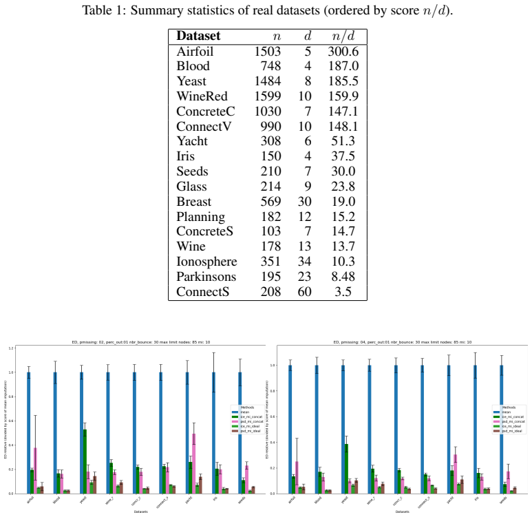
- [Figure 2] Figure 2 caption claims PSD-Impute “outperforms baselines by ≥15% on distributional metrics”; the plotted bars do not uniformly support a 15% relative improvement across all datasets and missing rates. Soften or quantify per-panel.
- [Abstract / §1] Several references to “classical minimax” and “beating the curse” appear before any rate is stated; a forward pointer to Theorem 5.4 (with the corrected wording) would avoid early over-claim.
- [Throughout / Appendix D] Typos: “regulirized” (§4), “dimen-sions” (§5.5), “T r” vs “Tr” inconsistency in Appendix D, and “ice_mi” in Figure 5 caption (presumably IterativeImputer MI).
- [§6.1] The complexity derivation in §6.1 quotes memory O(ε^{-24−10d/s}) for the SWM method; a short sanity check against the moderate-d regime used in experiments would make the asymptotic claim more credible.
Circularity Check
Minor non-load-bearing self-citation of PSD approximation theory from overlapping authors; the masked-risk ERM, learning-error bounds, and consistency derivation are independently developed and do not reduce to inputs by construction.
-
self citation load bearing
[§5.3 Theorem 5.1 and its proof sketch; also §4 (i)–(iv) and Appendix B.1–B.2]
"The theory of PSD models [26] tells us under assumption (i) it is possible to efficiently approximate a probability with a small mesh W, i.e. that there exists a good candidate Q̄ i R^{ℓ imesℓ}, Q̄≽0, such that p_Q̄ approximates very effectively p∗ and with a small Frobenius norm for Q̄. … When ℓ≥C1 ϵ^{-d/s}(log(C1/ϵδ))^{d/2}, η=C2 ϵ^{-2/s}/log(2/ϵ), then there exists Q̄ … ∥p_Q̄-p∗∥_{L2(Ω)}≤ϵ, tr(Q̄K)≤C3ℓ."
The existence of a low-complexity PSD approximant that underpins both the approximation-error bound (Thm 5.2) and the final rate (Thm 5.4) is taken from the authors' own prior paper [26] rather than re-derived from first principles. The citation is not circular in the strong sense (the prior theorem is independent of the imputation setting and supplies a genuine mathematical fact under the stated Hölder assumptions), yet it is the sole source of the approximation half of the excess-risk decomposition; without it the claimed rate would not follow. This is therefore a mild, non-load-bearing self-citation of the kind that scores 2.
full rationale
The paper's derivation chain is standard statistical learning: define masked KL risk L(p) whose zeros are exactly the distributions matching the observable marginals (Lemma 3.1), replace by the empirical negative log-likelihood of the masked observations (eq. 3), restrict to the PSD model class whose closed-form marginals make the problem convex (Thm 4.1), then bound excess risk by the usual approximation + generalization decomposition (eq. 6). The approximation half (Thm 5.1/B.1) imports the existence of a good PSD approximant from the authors' prior work [26], but that prior result is a general, parameter-free approximation theorem for Hölder densities under stated assumptions that do not mention imputation or the masked risk; the learning-error half (Thm 5.3), the balancing that produces the final rate (Thm 5.4), the interior-point solver, and the experimental protocol are all new and self-contained. No quantity is fitted to data and then re-presented as a prediction, no uniqueness theorem is imported to forbid alternatives, and the risk itself is not defined in terms of the estimator. The self-citation therefore raises the score only to the mild level of 2; the central consistency claim does not collapse by construction.
Assumptions & free parameters
free parameters (5)
- regularization λ (RKHS / trace term)
- mixture weight ν (uniform floor)
- barrier weight μ and schedule
- kernel precision η and anchor set W (size ℓ)
- smoothing α in log(Tr(QA_i)+α)
assumptions (5)
- domain assumption Missingness is MCAR: mask S is independent of X, so the joint factors as p⋆(x)⊗μ(S) (Section 3).
- domain assumption p⋆ is Hölder-s on a compact domain with s>d/2, bounded above, and either bounded away from zero or with zeros a C¹ manifold (Assumption 5.1(i)).
- standard math PSD kernel densities with Gaussian kernels have closed-form marginals and are dense in L¹ as anchors densify (properties from [17,26]).
- domain assumption Anchor mesh W is drawn uniformly i.i.d. on the hypercube (Assumption 5.1(ii)) so fill distance concentrates.
- ad hoc to paper KL is the right Bregman divergence for the empirical proxy (log-likelihood) of the masked risk (Section 3).
invented entities (1)
-
PSD-Impute estimator (p_Q with Q from regularized masked ERM)
Cite this review
Pith. "Pith review of Distributionally Faithful Imputation via Positive Semi-Definite Kernel Density Estimation." pith.science (2026). https://pith.science/paper/FKWRTKYP
@misc{pith2026260707767,
  author       = {Pith},
  title        = {Pith review of: Distributionally Faithful Imputation via Positive Semi-Definite Kernel Density Estimation},
  year         = {2026},
  howpublished = {\url{https://pith.science/paper/FKWRTKYP}},
  note         = {Machine review of arXiv:2607.07767}
}
read the original abstract
Missing values undermine statistical inference and machine learning pipelines, yet most imputation methods rely on heuristics or restrictive parametric assumptions that ignore the joint data distribution. We recast imputation under missing completely at random (MCAR) as density estimation from masked observations: estimate a distribution whose observed marginals exactly match those in the data. Leveraging positive semi definite (PSD) kernel densities we obtain a convex empirical risk problem with closed form marginals, solvable by a Newton interior point method. The resulting PSD Impute model yields both single and multiple imputations from the same fitted density, enjoys statistical consistency with fast adaptive excess risk beating the curse of dimensionality for very regular probabilities. Preliminary experiments on one synthetic and eleven real world datasets already indicate competitive distributional accuracy compared with popular imputation baselines, suggesting strong practical promise.
Figures


Figures from the paper (2 more)

Reference graph
Works this paper leans on
-
[1]
Springer Science & Business Media, 2013
Rajendra Bhatia.Matrix analysis. Springer Science & Business Media, 2013
work page 2013
-
[2]
Jeff A Bilmes et al. A gentle tutorial of the em algorithm and its application to parameter estimation for gaussian mixture and hidden markov models.International computer science institute, 4(510):126, 1998
work page 1998
-
[3]
Olivier Binette. A note on reverse pinsker inequalities.IEEE transactions on information theory, 65(7):4094–4096, 2019
work page 2019
-
[4]
Cambridge University Press, 2004
Stephen Boyd and Lieven Vandenberghe.Convex Optimization. Cambridge University Press, 2004
work page 2004
-
[5]
Alternating minimization as sequential unconstrained minimization: a survey
Charles L Byrne. Alternating minimization as sequential unconstrained minimization: a survey. Journal of Optimization Theory and Applications, 156:554–566, 2013
work page 2013
-
[6]
Thomas M Cover.Elements of information theory. John Wiley & Sons, 1999. 9
work page 1999
-
[7]
I-divergence geometry of probability distributions and minimization problems
Imre Csiszár. I-divergence geometry of probability distributions and minimization problems. The Annals of Probability, 3(1):146–158, 1975
work page 1975
-
[8]
Arthur P Dempster, Nan M Laird, and Donald B Rubin. Maximum likelihood from incomplete data via the em algorithm.Journal of the Royal Statistical Society: Series B (Methodological), 39(1):1–38, 1977
work page 1977
Show all 40 references
-
[9]
Matrix completion and low-rank svd via fast alternating least squares.Journal of Machine Learning Research, 16:3367–3402, 2015
Trevor Hastie, Rahul Mazumder, Jason Lee, and Reza Zadeh. Matrix completion and low-rank svd via fast alternating least squares.Journal of Machine Learning Research, 16:3367–3402, 2015
2015
-
[10]
On the consistency of supervised learning with missing values.Statistical Papers, 65(9):5447–5479, 2024
Julie Josse, Jacob M Chen, Nicolas Prost, Gaël Varoquaux, and Erwan Scornet. On the consistency of supervised learning with missing values.Statistical Papers, 65(9):5447–5479, 2024
2024
-
[11]
Regularization techniques for learning with matrices.The Journal of Machine Learning Research, 13(1):1865–1890, 2012
Sham M Kakade, Shai Shalev-Shwartz, and Ambuj Tewari. Regularization techniques for learning with matrices.The Journal of Machine Learning Research, 13(1):1865–1890, 2012
2012
-
[12]
Kingma and Jimmy Ba
Diederik P. Kingma and Jimmy Ba. Adam: A method for stochastic optimization. InInterna- tional Conference on Learning Representations, 2015
2015
-
[13]
Imputation for prediction: beware of diminishing returns.arXiv preprint arXiv:2407.19804, 2024
Marine Le Morvan and Gaël Varoquaux. Imputation for prediction: beware of diminishing returns.arXiv preprint arXiv:2407.19804, 2024
2024 arXiv
-
[14]
John Wiley and Sons, 3 edition, 2019
Roderick J A Little and Donald B Rubin.Statistical Analysis with Missing Data. John Wiley and Sons, 3 edition, 2019
2019
-
[15]
Explicit and recursive estimates of the lambert w function.arXiv preprint arXiv:2008.06122, 2020
Lajos Lóczi. Explicit and recursive estimates of the lambert w function.arXiv preprint arXiv:2008.06122, 2020
2008 arXiv
-
[16]
Vaem: a deep generative model for heterogeneous mixed type data.Advances in Neural Information Processing Systems, 33:11237–11247, 2020
Chao Ma, Sebastian Tschiatschek, Richard Turner, José Miguel Hernández-Lobato, and Cheng Zhang. Vaem: a deep generative model for heterogeneous mixed type data.Advances in Neural Information Processing Systems, 33:11237–11247, 2020
2020
-
[17]
Non-parametric models for non- negative functions.Advances in neural information processing systems, 33:12816–12826, 2020
Ulysse Marteau-Ferey, Francis Bach, and Alessandro Rudi. Non-parametric models for non- negative functions.Advances in neural information processing systems, 33:12816–12826, 2020
2020
-
[18]
Second order conditions to decom- pose smooth functions as sums of squares.SIAM Journal on Optimization, 34(1):616–641, 2024
Ulysse Marteau-Ferey, Francis Bach, and Alessandro Rudi. Second order conditions to decom- pose smooth functions as sums of squares.SIAM Journal on Optimization, 34(1):616–641, 2024
2024
-
[19]
Jared S. Murray. Multiple imputation: A review of practical and theoretical findings.Statistical Science, 33(2):142–159, 2018
2018
-
[20]
Missing data imputation using optimal transport
Boris Muzellec, Julie Josse, Claire Boyer, and Marco Cuturi. Missing data imputation using optimal transport. InInternational Conference on Machine Learning, pages 7130–7140. PMLR, 2020
2020
-
[21]
SIAM, 1994
Yurii Nesterov and Arkadii Nemirovskii.Interior-point polynomial algorithms in convex programming. SIAM, 1994
1994
-
[22]
What is a good imputation under mar missingness? arXiv preprint arXiv:2403.19196, 2024
Jeffrey Näf, Erwan Scornet, and Julie Josse. What is a good imputation under mar missingness? arXiv preprint arXiv:2403.19196, 2024
2024
-
[23]
Imputation scores.The Annals of Applied Statistics, 17(3):2452–2472, 2023
Jeffrey Näf, Meta-Lina Spohn, Loris Michel, and Nicolai Meinshausen. Imputation scores.The Annals of Applied Statistics, 17(3):2452–2472, 2023
2023
-
[24]
Multivariate beta distributions and independence properties of the wishart distribution.The Annals of Mathematical Statistics, pages 261–269, 1964
Ingram Olkin and Herman Rubin. Multivariate beta distributions and independence properties of the wishart distribution.The Annals of Mathematical Statistics, pages 261–269, 1964
1964
-
[25]
Scikit- learn: Machine learning in python.the Journal of machine Learning research, 12:2825–2830, 2011
Fabian Pedregosa, Gaël Varoquaux, Alexandre Gramfort, Vincent Michel, Bertrand Thirion, Olivier Grisel, Mathieu Blondel, Peter Prettenhofer, Ron Weiss, Vincent Dubourg, et al. Scikit- learn: Machine learning in python.the Journal of machine Learning research, 12:2825–2830, 2011. 10
2011
-
[26]
Psd representations for effective probability models
Alessandro Rudi and Carlo Ciliberto. Psd representations for effective probability models. Advances in Neural Information Processing Systems, 34:19411–19422, 2021
2021
-
[27]
Finding global minima via kernel approximations.arXiv preprint arXiv:2012.11978, 2020
Alessandro Rudi, Ulysse Marteau-Ferey, and Francis Bach. Finding global minima via kernel approximations.arXiv preprint arXiv:2012.11978, 2020
2012 arXiv
-
[28]
Cambridge University Press, 2014
Shai Shalev-Shwartz and Shai Ben-David.Understanding Machine Learning: From Theory to Algorithms. Cambridge University Press, 2014
2014
-
[29]
Sparse gaussian processes using pseudo-inputs
Edward Snelson and Zoubin Ghahramani. Sparse gaussian processes using pseudo-inputs. Advances in neural information processing systems, 18, 2005
2005
-
[30]
Missforest—non-parametric missing value imputation for mixed-type data.Bioinformatics, 28(1):112–118, 2012
Daniel J Stekhoven and Peter Bühlmann. Missforest—non-parametric missing value imputation for mixed-type data.Bioinformatics, 28(1):112–118, 2012
2012
-
[31]
The energy of data.Annual Review of Statistics and Its Application, 4(1):447–479, 2017
Gábor J Székely and Maria L Rizzo. The energy of data.Annual Review of Statistics and Its Application, 4(1):447–479, 2017
2017
-
[32]
Csdi: Conditional score-based diffusion models for probabilistic time series imputation.Advances in Neural Information Processing Systems, 34:24804–24816, 2021
Yusuke Tashiro, Jiaming Song, Yang Song, and Stefano Ermon. Csdi: Conditional score-based diffusion models for probabilistic time series imputation.Advances in Neural Information Processing Systems, 34:24804–24816, 2021
2021
-
[33]
Tsybakov.Introduction to Nonparametric Estimation
Alexander B. Tsybakov.Introduction to Nonparametric Estimation. Springer, 2009
2009
-
[34]
mice: Multivariate imputation by chained equations in r.Journal of Statistical Software, 45(3):1–67, 2011
Stef Van Buuren and Karin Groothuis-Oudshoorn. mice: Multivariate imputation by chained equations in r.Journal of Statistical Software, 45(3):1–67, 2011
2011
-
[35]
Springer, 2009
Cédric Villani.Optimal Transport: Old and New. Springer, 2009
2009
-
[36]
Are deep learning models superior for missing data imputation in large surveys? evidence from an empirical comparison
Zhenhua Wang, Olanrewaju Akande, Jason Poulos, and Fan Li. Are deep learning models superior for missing data imputation in large surveys? evidence from an empirical comparison. arXiv preprint arXiv:2103.09316, 2021
2021 arXiv
-
[37]
Numerical optimization, 2006
Stephen J Wright. Numerical optimization, 2006
2006
-
[38]
Gain: Missing data imputation using generative adversarial nets
Jinsung Yoon, James Jordon, and Mihaela van der Schaar. Gain: Missing data imputation using generative adversarial nets. InInternational Conference on Machine Learning, pages 5689–5698. PMLR, 2018. 11 Appendix of Distributionally Faithful Imputation via Positive Semi–Definite ...
2018
-
[39]
Our methodPSD_Imputeappears as a conditional mean estimator psd_mean and as a multiple imputer psd_multiple with m= 10 draws
and consists of iterative imputation by conditional mean expectation.SoftImpute[ 9] is a low-rank method that alternates between solving least-squares problems and applying singular value thresholding.OT[ 20] is an optimal transport based method, which minimizes a suitable met...
-
[40]
2.fort= 0,1,
InitialiseQ←I/ℓso thatTr(QH) = 1. 2.fort= 0,1, . . .do (a) Compute gradientand Hessian–vector products (b) Solve for Newton direction∆with SMW. (c) Newton decrementλ 2 =−⟨g(Q),∆⟩.ifλ 2/2≤εstop. (d) Backtracking line search: start α= 1 , reduce α←βα until f(Q+α∆) satisfies the ...
Reviewed July 10, 2026 · model on record in the stance chip above.
Discussion (0). Continue with ORCID to comment.