REVIEW 4 major objections 7 minor 26 references
Energy-Aware Model Predictive Control for Batch Manufacturing System Scheduling Under Different Electricity Pricing Strategies
T0 review · 4 major / 7 minor · reviewed 2026-08-06 · deepseek-v4-flash
Pith's one-line read This paper claims that a model predictive control scheduler repeatedly re-solving a mixed-integer quadratic program can adapt batch-manufacturing schedules to time-varying electricity prices, meeting daily production goals while cutting…
desk verdict Useful tariff-comparison case study, but the headline total-cost result is undermined by an objective that omits demand charges. read the letter →
The pith
A machine-rendered reading of the paper's core claim, the machinery that carries it, and where it could break.
The reading
What carries the argument
The load-bearing mechanism is the network-flow state-space model $x(k+1)=Ax(k)+Bu(k)+Ed(k)$, where nodes are buffers and edges are manufacturing processes, paired with binary activation variables $\delta_j(k)$ that encode machine on/off states and synchronization constraints for processes sharing a machine. The energy consumption model is $E(k)=\sum_{j}\varepsilon_j u_j(k)$, with $\varepsilon_j$ the power per unit processing rate, and only the energy usage charge enters the MPC objective; demand and basic charges are left out of the rolling optimization. The controller implements a shrinking horizon, solving the MIQP at each step and applying only the first optimal decision, while a time-varying production slack progressively tightens the requirement to hit the daily production goal.
What would settle it
Replace $E(k)=\sum_j \varepsilon_j u_j(k)$ with $E(k)=\sum_j \varepsilon_j u_j(k) + \sum_j \beta_j \delta_j(k)$ (adding a fixed power draw $\beta_j$ for each machine that is on) and rerun the 24-hour case study; if the total-cost ranking changes or the dynamic-pricing savings shrink, the linear-rate assumption drives the result.
Extended reading notes
Core claim
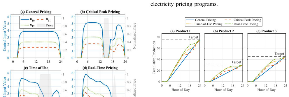
The central claim is that a receding-horizon optimization over a network model of buffers and processes, with an objective that penalizes buffer levels, schedule variation, production slack, and energy usage, produces schedules that automatically adapt to any electricity pricing structure. In the case study, critical peak, TOU, and real-time pricing concentrate production into low-price periods and avoid expensive hours, cutting energy usage charges by 14%, 11%, and 31% respectively compared with general pricing. Because operations are concentrated, peak power demand rises from 11.59 kW to 15.39, 16.63, and 17.73 kW under the three dynamic programs, which raises demand charges and partially offsets usage savings. Real-time pricing still achieves the lowest total cost at 109.02 USD (23% below general pricing), in part because its demand charge rate is roughly half that of the other programs. The paper states that this reveals a complex relationship between pricing structure and optimal scheduling, where simple load-shifting does not always minimize total cost when demand charges are significant.
Load-bearing premise
The energy model assumes machine power is linearly proportional to processing rate, with no fixed power draw, startup power, or standby power; if real machines consume significant energy just to be on or to ramp, the computed savings and the ranking of pricing programs can change.
Editorial extensions
If this is right
- Under critical peak, TOU, and real-time pricing, the MPC shifts production to low-price hours, cutting energy usage charges by 14%, 11%, and 31% relative to general pricing in the case study.
- The same load shifting raises peak power demand from 11.59 kW to 15.39, 16.63, and 17.73 kW, inflating demand charges under all dynamic pricing programs.
- Real-time pricing delivers the lowest total utility cost at 109.02 USD, a 23% reduction from general pricing, because its demand charge rate is about half that of the other programs.
- All pricing programs meet the daily production goals of 75, 30, and 45 units, with dynamic-pricing schedules showing stepped production that accelerates in cheaper hours.
- Manufacturers selecting among pricing programs should compare total cost, including demand charges, rather than energy usage charges alone.
Reading between the lines
- The paper's linear energy model omits fixed and transient power, so the reported savings are likely an upper bound; adding a per-on-state base power term would penalize frequent machine cycling and may favor flatter schedules.
- Because the demand charge is computed from the model's daily peak rather than a billing-monthly 15-minute peak, the total costs in Table IV are not directly comparable to actual utility bills, and the ranking could shift under the true billing interval.
- The same MIQP structure could be extended to coordinate on-site battery storage with production, allowing price arbitrage without the steep demand-charge penalty observed here.
- Running the controller with stochastic real-time prices rather than known day-ahead prices would test how much of the 23% saving survives forecast uncertainty.
Editorial analysis
A structured set of objections, weighed in public.
Referee Report
Summary. This paper develops a Model Predictive Control (MPC) framework for scheduling batch manufacturing systems under time-varying electricity prices. The manufacturing system is represented as a network of buffers and processes, with binary variables for machine activation and synchronization constraints for processes sharing a machine. The controller solves a Mixed-Integer Quadratic Program (MIQP) at each step that penalizes buffer levels, rate variations, production slack, and energy usage charges, with production goals enforced through time-varying soft constraints. A 24-hour case study compares general, critical peak, time-of-use, and real-time tariffs; the paper reports usage-charge reductions of 14%, 11%, and 31% for the dynamic tariffs and concludes that real-time pricing yields the lowest total cost (109.02 USD vs 141.16 USD for general pricing).
Significance. The paper addresses a relevant problem and provides a reasonably complete MIQP formulation with coupled machine groups and explicit parameters, which is a useful starting point for energy-aware MPC in batch manufacturing. The observation that load shifting to low-price periods can raise peak power and demand charges is worth stating. However, the paper's central quantitative claim--that real-time pricing is the best tariff under total cost--is not supported by the implemented controller, because the MPC objective omits demand charges while Table IV ranks tariffs by cost including them. The usage-charge savings are near-tautological consequences of the objective, whereas the more interesting demand-charge tradeoff is an artifact of the unmodeled peak term. With a demand-aware objective or a clarified scoping of the claims, the framework could be a useful comparative tool.
major comments (4)
- [§IV.D, Eq. (22); §V.B, Table IV] The MPC objective in Eq. (22) minimizes only ω_e·C_energy plus buffer, rate-variation, and slack terms, and Section IV.D explicitly states that demand and basic charges are not considered. Table IV nevertheless ranks tariffs by total cost computed from Eq. (8), which includes the demand charge ρ_d·max_k E(k) and basic charge ρ_b·N. Since the demand charge depends on the peak of E(k), it is not a constant offset like the basic charge; omitting it from the objective means the reported total-cost ordering is not a consequence of the optimization. A demand-aware controller could accept a slightly higher usage charge to shave the peak and reverse the ranking (e.g., real-time pricing has peak 17.73 kW vs 11.59 kW under general pricing). The authors should either add a demand-charge term to the MIQP (e.g., via an epigraph variable for peak power) or explicitly limit the claims to usage-charge minimization and treat Table IV as an ex-post accounting exercise.
- [§II (Problem Statement) vs §IV.D] The problem statement says the goal is to 'minimize the total energy cost incurred throughout the production process,' but the implemented objective omits demand charges while the basic charge, being constant over a fixed horizon, would not affect the schedule. This is an internal inconsistency: the demand charge is schedule-dependent and should appear in the objective if total cost is the stated goal. The paper should reconcile the two, for example by redefining the problem statement to target usage charges or by extending the objective.
- [§V.B, Table IV and Figs. 4-5] The finding that dynamic pricing raises peak power and can increase demand charges is presented as a key insight. However, with a usage-only objective, concentrating production in low-price periods is the expected and designed behavior, so the higher peaks do not demonstrate a tradeoff that the controller has weighed; they are simply the unpenalized side effect. To make the claimed practical insight ('intuitive approaches of shifting operations to lower-rate periods may not always yield the lowest total cost') credible, the paper needs at least one experiment in which the controller accounts for peak power, or a post-hoc analysis showing that no peak-shaving modification within a reasonable usage-cost sacrifice changes the ranking.
- [§II Assumption (3); Eq. (7)] The energy model E(k)=Σ_{j=1}^{n_u} ε_j u_j(k) contains no fixed-power or standby-power term, even though binary activation variables δ_j(k) are available and machines are turned on and off throughout the day. In batch manufacturing, fixed and transient power consumption is often substantial, and adding a term such as ε_fixed δ_j(k) would change the optimal timing of machine starts and stops, and therefore the demand/usage tradeoff and the tariff ranking. The authors should either extend the energy model with a fixed-power term or provide a sensitivity discussion showing that the qualitative conclusion is robust to this simplification.
minor comments (7)
- [Eq. (16)] In Eq. (16), the summation variable should be d_p(t), not d_p(k), to avoid confusion with the current step.
- [Eq. (8)] The text '∀k = 0, 2, ..., N − 1' should read '∀k = 0, 1, ..., N − 1' to match the summation range.
- [Table III] Table III lists 'u1,...,12 min 0 units/hour' twice; the second row should presumably be 'u1,...,12 max' or the intended maximum flow value, and the table should be corrected.
- [Eqs. (7) and (14)] The symbol ε is used both for the energy coefficient in Eq. (7) and for the minimum flow rate in Eq. (14); this notation should be disambiguated (e.g., using ε_min for the latter), especially since Table III also uses ε for energy coefficients.
- [Eq. (22) vs Eqs. (17)-(19)] The slack penalty in Eq. (22) is written as s_j(k) with j=1..n_d, while Eqs. (17)-(19) define s_p(k) indexed by product; the notation should be aligned.
- [Eqs. (20)-(21)] The relationship between h (production time step) and k (MPC prediction step) is not defined; please clarify how α(k) is updated in the closed-loop shrinking-horizon implementation.
- [Fig. 6 caption] The caption contains the typo 'differenrt'; it should read 'different'.
Circularity Check
No circular derivation: the cost comparisons are emergent outputs of a self-contained MPC simulation, with no fitted parameter or self-citation chain doing the work.
full rationale
The paper's derivation is self-contained. The MIQP in Eq. (22) minimizes a weighted combination of buffer, rate-variation, slack, and energy-usage terms; the reported energy-usage costs in Table IV are the C_energy terms that the controller optimizes, so reporting that dynamic pricing lowers usage charges is a demonstration that the optimizer responds to price signals, not a fitted input renamed as a prediction. The non-trivial total-cost ranking (real-time pricing lowest at 109.02 USD despite the highest peak power) emerges from applying demand and basic charges from Eq. (8) after the fact; Section IV.D explicitly states that demand and basic charges are not in the MPC objective. That mismatch is a modeling-scope and correctness concern, not circularity: the ranking is not forced by construction, and in fact the demand-charge term works against the controller's usage-minimizing choices. The only self-citations are to the authors' prior CASE 2023 framework [5], used as background and motivation; no load-bearing premise, uniqueness theorem, or ansatz is imported from it. The energy model (linear rate-power assumption, Eq. (7)) and the ComEd/PJM pricing data are external inputs, not outputs of the claimed result. No step of the derivation reduces to its own inputs, so no circularity is identified.
Assumptions & free parameters
free parameters (8)
- omega_x =
1
- omega_u =
0.5
- omega_s =
1000
- omega_e =
500
- tau (base production tolerance) =
0.05
- xi (tightening factor) =
0.5
- Lambda (big-M) =
unspecified
- epsilon_min (minimum flow rate) =
unspecified
assumptions (6)
- domain assumption Process yield rate is not considered (A is the identity matrix).
- domain assumption The system has unlimited raw materials for production.
- domain assumption Each product has a daily production goal known a day ahead.
- domain assumption Machine power is linearly related to the processing rate with no fixed power draw.
- domain assumption Demand charge is computed on peak power over the control horizon N, not the true billing period.
- ad hoc to paper The tolerance schedule alpha(k) = tau times (1 - eta(k)(1 - xi)) is a valid proxy for production deadline pressure.
Cite this review
Pith. "Pith review of Energy-Aware Model Predictive Control for Batch Manufacturing System Scheduling Under Different Electricity Pricing Strategies." pith.science (2026). https://pith.science/paper/FLFWEAXM
@misc{pith2026250622923,
  author       = {Pith},
  title        = {Pith review of: Energy-Aware Model Predictive Control for Batch Manufacturing System Scheduling Under Different Electricity Pricing Strategies},
  year         = {2026},
  howpublished = {\url{https://pith.science/paper/FLFWEAXM}},
  note         = {Machine review of arXiv:2506.22923}
}
read the original abstract
Manufacturing industries are among the highest energy-consuming sectors, facing increasing pressure to reduce energy costs. This paper presents an energy-aware Model Predictive Control (MPC) framework to dynamically schedule manufacturing processes in response to time-varying electricity prices without compromising production goals or violating production constraints. A network-based manufacturing system model is developed to capture complex material flows, batch processing, and capacities of buffers and machines. The scheduling problem is formulated as a Mixed-Integer Quadratic Program (MIQP) that balances energy costs, buffer levels, and production requirements. A case study evaluates the proposed MPC framework under four industrial electricity pricing schemes. Numerical results demonstrate that the approach reduces energy usage expenses while satisfying production goals and adhering to production constraints. The findings highlight the importance of considering the detailed electricity cost structure in manufacturing scheduling decisions and provide practical insights for manufacturers when selecting among different electricity pricing strategies.
Figures


Figures from the paper (2 more)

Reference graph
Works this paper leans on
-
[1]
Algorithms for nest ing problems,
J. F. C. Oliveira and J. A. Ferreira, “Algorithms for nest ing problems,” in Applied Simulated Annealing , R. V . Vidal, Ed. Berlin, Germany: Springer, 1993, pp. 255–273
work page 1993
-
[2]
IECL: an intel ligent en- ergy consumption model for cloud manufacturing,
Z. Zhou, M. Shojafar, M. Alazab, and F. Li, “IECL: an intel ligent en- ergy consumption model for cloud manufacturing,” IEEE Transactions on Industrial Informatics , vol. 18, no. 12, pp. 8967–8976, 2022
work page 2022
-
[3]
Use of Energy in the Industry Sector,
U.S. Energy Information Administration, “Use of Energy in the Industry Sector,” 2025. [Online]. Available: https://www .eia.gov
work page 2025
-
[4]
Toward intelligent machine-to-machine commun ications in smart grid,
Z. M. Fadlullah, M. M. Fouda, N. Kato, A. Takeuchi, N. Iwas aki, and Y . Nozaki, “Toward intelligent machine-to-machine commun ications in smart grid,” IEEE Communications Magazine , vol. 49, no. 4, pp. 60–65, 2011
work page 2011
-
[5]
H. Li, H. C. Pangborn, and I. Kovalenko, “A system-level e nergy- efficient digital twin framework for runtime control of batc h manu- facturing processes,” in 2023 IEEE 19th International Conference on Automation Science and Engineering (CASE) , 2023, pp. 1–6
work page 2023
-
[6]
M. L. Pinedo, Scheduling: Theory, Algorithms, and Systems , 5th ed. New Y ork, NY , USA: Springer, 2016
work page 2016
-
[7]
Real-time schedul ing of cloud manufacturing services based on dynamic data-driven simula- tion,
L. Zhou, L. Zhang, L. Ren, and J. Wang, “Real-time schedul ing of cloud manufacturing services based on dynamic data-driven simula- tion,” IEEE Transactions on Industrial Informatics , vol. 15, no. 9, pp. 5042–5051, 2019
work page 2019
-
[8]
W. Shao, Z. Shao, and D. Pi, “An ant colony optimization be havior- based moea/d for distributed heterogeneous hybrid flow shop schedul- ing problem under nonidentical time-of-use electricity ta riffs,” IEEE Transactions on Automation Science and Engineering , vol. 19, no. 4, pp. 3379–3394, 2021
work page 2021
Show all 26 references
-
[9]
C ooperative product agents to improve manufacturing system flexibility : A model- based decision framework,
I. Kovalenko, E. C. Balta, D. M. Tilbury, and K. Barton, “C ooperative product agents to improve manufacturing system flexibility : A model- based decision framework,” IEEE Transactions on Automation Science and Engineering , vol. 20, no. 1, pp. 440–457, 2023
2023
-
[10]
Industry 4.0 and industry 5.0—inception, conception and perception,
X. Xu, Y . Lu, B. V ogel-Heuser, and L. Wang, “Industry 4.0 and industry 5.0—inception, conception and perception,” Journal of Man- ufacturing Systems , vol. 61, pp. 530–535, 2021
2021
-
[11]
A new app roach to scheduling in manufacturing for power consumption and ca rbon footprint reduction,
K. Fang, N. Uhan, F. Zhao, and J. W. Sutherland, “A new app roach to scheduling in manufacturing for power consumption and ca rbon footprint reduction,” Journal of Manufacturing Systems , vol. 30, no. 4, pp. 234–240, Oct. 2011
2011
-
[12]
Operational m ethods for minimization of energy consumption of manufacturing eq uipment,
G. Mouzon, M. B. Yildirim, and J. Twomey, “Operational m ethods for minimization of energy consumption of manufacturing eq uipment,” International Journal of Production Research , vol. 45, no. 18-19, pp. 4247–4271, Sep. 2007
2007
-
[13]
Optimizing the production scheduling of a single mac hine to minimize total energy consumption costs,
F. Shrouf, J. Ordieres-Meré, A. García-Sánchez, and M. Ortega- Mier, “Optimizing the production scheduling of a single mac hine to minimize total energy consumption costs,” Journal of Cleaner Production, vol. 67, pp. 197–207, Mar. 2014
2014
-
[14]
An overview of industrial m odel predictive control technology,
S. J. Qin and T. A. Badgwell, “An overview of industrial m odel predictive control technology,” in AIche Symposium Series , vol. 93. American Institute of Chemical Engineers, 1997, pp. 232–25 6
1997
-
[15]
Constrained model predictive control: Stability and opti mality,
D. Q. Mayne, J. B. Rawlings, C. V . Rao, and P . O. M. Scokaer t, “Constrained model predictive control: Stability and opti mality,” Au- tomatica, vol. 36, no. 6, pp. 789–814, Jun. 2000
2000
-
[16]
Integrated production s cheduling and process control: A systematic review,
M. Baldea and I. Harjunkoski, “Integrated production s cheduling and process control: A systematic review,” Computers & Chemical Engineering, vol. 71, pp. 377–390, Dec. 2014
2014
-
[17]
An energy-awa re mul- tiobjective optimization framework to minimize total tard iness and energy cost on a single-machine nonpreemptive scheduling,
S. Rubaiee, S. Cinar, and M. B. Yildirim, “An energy-awa re mul- tiobjective optimization framework to minimize total tard iness and energy cost on a single-machine nonpreemptive scheduling, ” IEEE Transactions on Engineering Management , vol. 66, no. 4, pp. 699– 714, 2018
2018
-
[18]
Model predictive control of priced timed automata encoded with first-order logic,
E. C. Balta, I. Kovalenko, I. A. Spiegel, D. M. Tilbury, a nd K. Barton, “Model predictive control of priced timed automata encoded with first-order logic,” IEEE Transactions on Control Systems Technology , vol. 30, no. 1, pp. 352–359, 2022
2022
-
[19]
Exact and heuris tic solution approaches for energy-efficient identical parallel machin e scheduling with time-of-use costs,
M. Gaggero, M. Paolucci, and R. Ronco, “Exact and heuris tic solution approaches for energy-efficient identical parallel machin e scheduling with time-of-use costs,” European Journal of Operational Research , vol. 311, no. 3, pp. 845–866, 2023
2023
-
[20]
(2023) Comed
Commonwealth Edison Company (ComEd). (2023) Comed. [O nline]. Available: https://www.comed.com/
2023
-
[21]
(2023) Pjm your power our gri d
PJM Interconnection, LLC. (2023) Pjm your power our gri d. [Online]. Available: https://www.pjm.com/
2023
-
[22]
(2023) O pen energy information
National Renewable Energy Laboratory (NREL). (2023) O pen energy information. [Online]. Available: https://openei.org
2023
-
[23]
MA TLAB version (R2023a),
The MathWorks Inc., “MA TLAB version (R2023a),” Natick , Massachusetts, United States, 2023. [Online]. Available: https: //www.mathworks.com
2023
-
[24]
Y ALMIP: A toolbox for modeling and optimiz ation in MA TLAB,
J. Löfberg, “Y ALMIP: A toolbox for modeling and optimiz ation in MA TLAB,” in In Proceedings of the CACSD Conference , Taipei, Taiwan, 2004
2004
-
[25]
GUROBI Optimizer Referenc e Manual,
GUROBI Optimization, LLC, “GUROBI Optimizer Referenc e Manual,” 2024. [Online]. Available: https://www.gurobi. com
2024
-
[26]
Optimal economic schedule for a network of microgrids with hybrid energy stor age system using distributed model predictive control,
F. Garcia-Torres, C. Bordons, and M. A. Ridao, “Optimal economic schedule for a network of microgrids with hybrid energy stor age system using distributed model predictive control,” IEEE Transactions on Industrial Electronics , vol. 66, no. 3, pp. 1919–1929, 2018
1919
Reviewed August 6, 2026 · model on record in the stance chip above.
Discussion (0). Continue with ORCID to comment.