REVIEW 2 major objections 5 minor 19 references
Theoretical Learning Performance of Graph Neural Networks: The Impact of Jumping Connections and Layer-wise Sparsification
T0 review · 2 major / 5 minor · reviewed 2026-08-06 · deepseek-v4-flash
Pith's one-line read The paper proves that a two-hidden-layer GCN with a jumping connection, trained by SGD with layer-wise edge pruning, matches the best achievable prediction error in its target class — and that the second layer tolerates far more…
desk verdict First rigorous treatment of layer-wise sparsification with jump connections, but the asymmetry result is purchased by a small-α assumption the experiments never probe. read the letter →
The pith
A machine-rendered reading of the paper's core claim, the machinery that carries it, and where it could break.
The reading
What carries the argument
The argument rides on three coupled objects. The first is the sparse effective adjacency matrix $A^*$: formed by keeping only the largest entries in each block of the normalized adjacency matrix, it identifies the edges that carry meaningful message propagation, and the analysis shows that sparsified training matrices need only stay close to $A^*$ rather than to the full adjacency matrix $A$. The second is the concept class $H = F + \alpha G(F)$, a hierarchy in which the first hidden layer learns a simpler, dominant base function $F$ and the second hidden layer learns a composite correction $G(F)$ scaled by a small weight $\alpha$; this magnitude ordering is what makes the second layer's sparsification error tolerable. The third is a proof skeleton for three-layer ReLU networks with random initialization — weight deviations from initialization, coupling lemmas for how ReLU activation patterns change, and gradient-concentration estimates — extended to semi-supervised node regression where labels depend on neighboring features and adjacency matrices are sparsified. The per-layer deviation bounds of Lemma 3.1 convert control of $\|A_t^1 - A^*\|_1$ and $\|A_t^2 - A^*\|_1$ into the claimed output error.
What would settle it
Train the same two-hidden-layer architecture on synthetic targets where the composite term's magnitude $\alpha$ is order 1 rather than order $1/C_s(G)$, so the second layer contributes as much as the first: the theorem's error term $\varepsilon_0 = \tilde{O}(\alpha^4 C_s(G)^4)$ then saturates, and the theory predicts that the layer-wise pruning asymmetry shrinks and the second layer's extra pruning tolerance disappears — observing the asymmetry persist at large $\alpha$ would contradict the paper's account of what causes it.
Extended reading notes
Core claim
On its own terms, the paper claims that a two-hidden-layer GCN with a single jumping connection, re-parameterized so only the first-layer weight $W$ and second-layer weight $V$ are learned, is trainable by SGD with a degree-aware edge-pruning schedule. In Theorem 3.2, for $\alpha \in (0, \tilde{O}(1/C_s(G)))$ and pruning probabilities satisfying (12), once the width $m$, iteration count $T$, and labeled set $|\Omega|$ are large enough, the iterates satisfy $$\frac{1}{T}\sum_{t=0}^{T-1} \mathbb{E}\,\|y_n - \mathrm{out}_n(X, $A_t^{1}$, $A_t^{2}$; W_t, V_t)\|^2 \le \varepsilon$$ with $\varepsilon = 10\cdot\mathrm{OPT} + \tilde{O}(\alpha^4 C_s(G)^4)$, where OPT is the smallest error in the concept class $H = F + \alpha G(F)$ evaluated with $A^*$. The structural claim is Lemma 3.1: the two sparsified layers' deviations from $A^*$ are controlled separately, and because the second layer's contribution is weighted by the small $\alpha$, its pruning probability $p^2_{ij}$ may be larger than $p^1_{ij}$ while the output error stays bounded. The paper reads this as the jumping connection decoupling the layers, so sparsification requirements differ across layers.
Load-bearing premise
The load-bearing premise is that the true node-label function is dominated by a simple base function, with the more complex composite part contributing only a small amount; the paper's conclusion that the second layer tolerates more aggressive pruning rests on this magnitude ordering rather than on the jumping connection alone, and the paper gives no evidence beyond its own synthetic construction that real node-label functions actually have this structure.
Editorial extensions
If this is right
- In a two-hidden-layer GCN with a jumping connection, pruning in the first layer must be conservative while the second layer can be pruned far more aggressively, with the same output error guarantee.
- Sparsified training matrices need only approximate $A^*$, not the original adjacency matrix $A$, so very sparse graphs can match the accuracy of the full graph when $A^*$ captures the informative edges.
- The sample complexity scales as $\tilde{O}(\log N)$ labeled nodes, so a logarithmic number of labels can suffice to generalize across the whole graph under the paper's assumptions.
- A denser effective matrix (larger $\|A^*\|_1$) provably requires more neurons and more labels to reach the same test error, which the paper also confirms in experiments by varying the degree distribution.
- The generalization bound tracks OPT, the best error in the target class: the learned model's accuracy is near-optimal for the function class, so the practical quality of the model is governed by how well the class captures the true node-label mapping.
Reading between the lines
- The layer-wise asymmetry is formally driven by the smallness of $\alpha$, the weight of the composite term, rather than by the jumping connection alone; an experiment sweeping $\alpha$ from tiny to order one would separate the two causes, since the paper's own bounds predict the extra pruning tolerance of the second layer shrinks as $\alpha$ grows.
- The experiments on 8-layer and 4-layer Jumping Knowledge Networks suggest the layer-wise principle transfers to deeper stacks, but the proof covers only two hidden layers; whether cumulative sparsification errors in deeper architectures preserve the asymmetry is a natural, still-open test.
- The empirical evaluation includes dropout and normalization layers that the theory does not model, so those experiments are confirmatory in spirit rather than a direct check of the theorem's conditions.
- The $A^*$ viewpoint yields a practical diagnostic: pruning algorithms that preserve the blocks of low-degree edges that define $A^*$'s retained entries should degrade generalization least, and measuring a pruned graph's deviation from $A^*$ rather than from $A$ could predict which sparse graphs stay accurate.
Editorial analysis
A structured set of objections, weighed in public.
Referee Report
Summary. This paper presents a theoretical analysis of training a two-hidden-layer GCN with a single jumping connection by SGD under layer-wise edge sparsification. The authors introduce a block-wise, degree-aware pruning rule and a sparse effective adjacency matrix A* defined by the top entries of the normalized adjacency matrix within each degree block. The target concept class is H = F_{A*} + αG_{A*}(F_{A*}), where F and G are one-hidden-layer GCNs with smooth activations and α is assumed small relative to 1/Cs(G). Lemma 3.1 bounds the output error caused by sparsified matrices A1t, A2t in terms of their ℓ1 deviations from A*, with the first-layer tolerance scaled by 1/Cs(F) and the second-layer tolerance scaled by 1/(αCs(F)Cs(G)). Theorem 3.2 then provides a bound ε = 10·OPT + ε0 on the time-averaged prediction error, with explicit model, iteration, and sample complexities, implying that the learned model nearly matches the best achievable error in the concept class. The paper's headline qualitative claim is that the second hidden layer can tolerate more aggressive sparsification than the first. The theory is accompanied by synthetic experiments and OGB experiments on deep Jumping-Knowledge GCNs.
Significance. If the results hold, this is a useful contribution: it extends the training-dynamics-plus-generalization analysis of Li et al. (2022a) and Zhang et al. (2023b) to architectures with jumping connections, provides explicit sample complexity for a sparsified GCN, and makes falsifiable predictions (the layer-wise asymmetry; the ∥A*∥1-dependence of model and sample complexity) that the experiments address. Credit is due for the transparency of the assumptions: the concept class and the small-α condition are stated explicitly rather than hidden, and the qualitative prediction is tested on real datasets. Two caveats temper the significance. First, A* is defined by the same degree-aware top-entry rule that the sampling strategy assumes, so the descriptive claim that 'sparsification works when A_t stays close to A*' is partly a statement about concentration around the rule's canonical sparse matrix. Second, the central asymmetry is mathematically driven by the assumed magnitude hierarchy of the two target components, so the architectural attribution of the effect requires the robustness check described in the major comments.
major comments (2)
- [§3.2, Lemma 3.1, Eq. (12); §4.1] The paper's headline claim—that jumping connections make deeper layers more tolerant of sparsification—is stated in the abstract and in contribution (3) as a property of the architecture. As proved, however, the asymmetry p2_ij > p1_ij in Eq. (12) is a direct algebraic consequence of the small-α assumption αCs(G) < 1 in the denominator of the p2 bound, together with the weight bound ‖Vt‖ ≤ Θ̃(αCs(G)) in Table 3; the jumping connection makes the loss decomposable, but the direction of the inequality is set by the target-magnitude ordering H = F + αG(F). If αCs(G) ≥ 1, Eq. (12) gives p2_ij ≤ p1_ij and the second-layer tolerance (14) shrinks below the first layer's, with the jumping connection still present. The claim should therefore be either reformulated as conditional on the composite term being small, or made robust by evidence: the synthetic experiments in Section 4.1 use only α = 0.5, and no experiment varies α or compares against a target with αCs(G) ≥ 1. A sweep over α in the synthetic layer-wise experiment would directly test whether the qualitative conclusion is attributable to the architecture or to the assumed magnitude ordering.
- [Appendix C.2, proof of Lemma C.2] The proof of the key existence lemma invokes 'Lemma E.1. from?' without stating the lemma or giving a citation. Lemma C.2 is the basis for Lemma C.3, which supplies the reference weights W*, V* used in the first term of the error decomposition (18) and hence is load-bearing for Theorem 3.2. The missing lemma must be stated or properly cited before the proof can be considered complete.
minor comments (5)
- [Appendix C.5, Lemma C.7] Equations (85) and (86) state the probability of the good event (small deviation) as Pr[‖A1t − A*‖1 ≤ O(‖Errt‖/τw)] ≤ e^{−Ω(...)}, which is the wrong direction; the proof bounds the complementary upper-tail event, so these displays should read ≥ 1 − e^{−Ω(...)}. As printed, the lemma contradicts its use in the proof of Theorem 3.2.
- [§4.3] The interpretation that 'multiple sparse A*' may exist for different (q1, q2) pairs is speculative; the theory fixes a single A* by the block-wise top-entry rule, and the experiments do not measure ‖A1t − A*‖1 or ‖A2t − A*‖1, so this explanation is not grounded in the formal results.
- [§1.1] 'neural tangent kennel' should be 'neural tangent kernel'.
- [§3.2 / §4.1] The map between the theoretical sampling objects (block-wise top d1√(di/dj) entries, probabilities p1_ij, p2_ij) and the algorithm/experiments (top-q1 and top-q2 fractions retained with 99%/1% probabilities) is never made formal; stating how q1 and q2 relate to p1_ij and p2_ij would tighten the link between Theorem 3.2 and the empirical results.
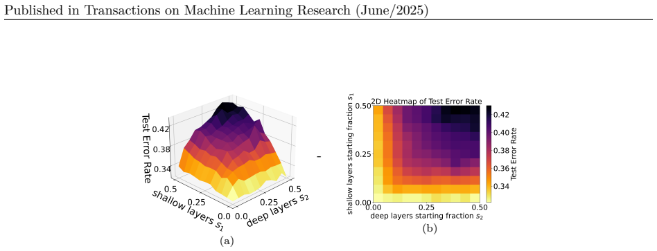
- [Figures 1 and 2] These figures validate the ∥A*∥1 dependence of model and sample complexity by training directly with A*, rather than by comparing SGD with sampled A1t, A2t against training with A*; the claim that sparsified training matches A*-training is therefore tested only indirectly (Figure 3 and the OGB experiments, which use a simplified sampling rule).
Circularity Check
The layer-wise sparsification asymmetry is a restatement of the small-α target assumption, and A* is defined by the paper's own pruning rule; the main error bound is proved but the headline qualitative claim reduces by construction.
-
self definitional
[Section 3.3 (Concept Class) and Lemma 3.1 / Eq. (12)]
"We assume 0<α≤~O(1/Cs(G)) throughout the training. ... since ~Θ(αCs(G))<1 (see Table 3 in the Appendix), the second-layer sparsification condition in (12) permits larger values of p2_ij compared to p1_ij, allowing more aggressive pruning in the second layer while still satisfying the output error bound in (15)."
Equation (12) makes p1_ij ≤ ~Θ(√didjE/(NiNjCs(F))) and p2_ij ≤ ~Θ(√didjE/(NiNjαCs(F)Cs(G))), so p2_ij > p1_ij is algebraically equivalent to αCs(G)<1, which is exactly the paper's stated assumption that the composite term αG(F) contributes less than F. The larger second-layer deviation tolerance in (14) is similarly the reciprocal of the same small-α assumption. Thus the central claim that 'jumping connections lead to different sparsification requirements across layers' is a restatement of the target-magnitude ordering rather than an independent consequence of the architecture; if αCs(G)≥1, the inequality reverses and the claimed asymmetry disappears even with the jump connection intact.
-
self definitional
[Section 3.2 (definition of A*) and Lemma 3.1]
"To analyze the impact of this graph topology sparsification on the learning performance, we define the sparse effective adjacency matrix A* where in each submatrix A*_Bij: (1) if i>j, the top d1 sqrt(di/dj) largest values in A_Bij remain the same, while other entries are set to zero. ... If i > j, each of the top 2 d1 sqrt(di/dj) largest entries A_ij in A_Bij is retained independently with high probability 1-p^k_ij."
A* is defined as the deterministic limit of the paper's own sampling rule, which retains exactly those top entries with high probability. Lemma 3.1 then bounds ||A1t - A*||_1 under condition (12), so the conclusion that graph sparsification preserves generalization whenever the sampled matrices stay close to A* is true by construction of A*. The crucial input that A* preserves 'essential edges' is not established independently; synthetic labels are generated using this same A*, so the validation does not test the condition against data. This is a definitional feature rather than a fitted loop, but it makes that part of the framing tautological.
full rationale
The core Theorem 3.2 is a genuine proof: the SGD generalization bound is derived from explicit assumptions and does not fit any parameter to test data, so the numerical error guarantee is not circular. However, the paper's headline qualitative claim—that jumping connections make the second layer tolerate more sparsification than the first—reduces by construction to the small-α assumption in the concept class H = F + αG(F). Equation (12) makes p2/p1 = Θ(1/(αCs(G))), so the asserted p2 > p1 and the larger allowed deviation (14) are algebraic restatements of αCs(G) < 1; if that inequality is violated, the asymmetry reverses. Additionally, A* is defined as the deterministic version of the paper's own pruning rule, so the statement that sparsification works when As stays close to A* is partly true by definition. These are explicit conditions, not hidden fits, and the main proof retains independent content; the circularity is localized to the interpretation of the layer-wise asymmetry as an architecture-driven discovery.
Assumptions & free parameters
free parameters (3)
- alpha (α) =
≤ Õ(1/Cs(G)) in theory; 0.5 in synthetic experiments
- Top-k thresholds for A* =
d1√(di/dj) (i>j) and d1 (i≤j)
- Initialization variances σ_w, σ_v =
σ_w ∈ [m^{-1/2+0.01}, m^{-0.01}], σ_v = Θ(polylog(m))
assumptions (6)
- domain assumption Node degrees can be grouped into L groups with degrees of the same order d_l, and d_l = o(d_{l+1})
- domain assumption Target functions F and G are smooth with bounded model/sample complexity (Cs, Cm); G is LG-Lipschitz
- ad hoc to paper The weight α of the composite term is small: α ≤ Õ(1/(k p_G Cs(G, BF||A*||_1)))
- domain assumption Minimum degree δ(G) ≥ Ω(||Err_t||/τ_w) (Lemma C.7)
- domain assumption Maximum degree Δ ≤ O((Nε^2)^{1/4}) and sample size |Ω| large (Lemma C.8)
- standard math C fixed at random initialization; W0, V0 Gaussian with specified variances
invented entities (1)
-
Sparse effective adjacency matrix A*
Cite this review
Pith. "Pith review of Theoretical Learning Performance of Graph Neural Networks: The Impact of Jumping Connections and Layer-wise Sparsification." pith.science (2026). https://pith.science/paper/FMNDIMFS
@misc{pith2026250705533,
  author       = {Pith},
  title        = {Pith review of: Theoretical Learning Performance of Graph Neural Networks: The Impact of Jumping Connections and Layer-wise Sparsification},
  year         = {2026},
  howpublished = {\url{https://pith.science/paper/FMNDIMFS}},
  note         = {Machine review of arXiv:2507.05533}
}
abstract
Jumping connections enable Graph Convolutional Networks (GCNs) to overcome over-smoothing, while graph sparsification reduces computational demands by selecting a sub-matrix of the graph adjacency matrix during neighborhood aggregation. Learning GCNs with graph sparsification has shown empirical success across various applications, but a theoretical understanding of the generalization guarantees remains limited, with existing analyses ignoring either graph sparsification or jumping connections. This paper presents the first learning dynamics and generalization analysis of GCNs with jumping connections using graph sparsification. Our analysis demonstrates that the generalization accuracy of the learned model closely approximates the highest achievable accuracy within a broad class of target functions dependent on the proposed sparse effective adjacency matrix $A^*$. Thus, graph sparsification maintains generalization performance when $A^*$ preserves the essential edges that support meaningful message propagation. We reveal that jumping connections lead to different sparsification requirements across layers. In a two-hidden-layer GCN, the generalization is more affected by the sparsified matrix deviations from $A^*$ of the first layer than the second layer. To the best of our knowledge, this marks the first theoretical characterization of jumping connections' role in sparsification requirements. We validate our theoretical results on benchmark datasets in deep GCNs.
Figures


Figures from the paper (4 more)



Reference graph
Works this paper leans on
-
[1]
‖‖CDn W+W0 WXan−CDn W+W0 (W+W 0)Xan ‖‖ 2≤ ~O (√s√mτw∥A∥1 + √ kσw∥A∥1 ) (29)
‖‖Dn W(0)−Dn W+W0 ‖‖ 0≤O ( (τw σw )2/3m2/3 ) (28) 2. ‖‖CDn W+W0 WXan−CDn W+W0 (W+W 0)Xan ‖‖ 2≤ ~O (√s√mτw∥A∥1 + √ kσw∥A∥1 ) (29)
-
[2]
We writeCD n W+W0 WXa∗1 n −CD n W+W0 (W+W 0)Xa∗1 n =−CD n W0 W(0)Xa∗1 n + C ( Dn W0−Dn W+W0 ) W0Xa∗1 n . For the first term, ‖‖Dn W0 W0Xan ‖‖ 2 ≤ ∥W 0Xan∥2 ≤ O(σw∥A∥1 √m), so ‖‖CDn W0 W0Xan ‖‖ 2≤ ~O (√ kσw∥A∥1 ) For the second term, using Lemma A.2 again, we have ‖‖( Dn W0−Dn W+W0 ) W0Xan ‖‖ 2≤∥WXa n∥2≤τ w∥A∥1 Using Lemma A.1, for everys-sparse vectory, i...
-
[3]
‖‖Dn V(0)−Dn V+V0 ‖‖ 0≤O ( (τv σv )2/3m ) (31)
‖‖out1 n(X,A;W) ‖‖ 2≤ ~O(τw∥A∥1)(30) 4. ‖‖Dn V(0)−Dn V+V0 ‖‖ 0≤O ( (τv σv )2/3m ) (31)
-
[4]
Similar to (28), ‖‖Vout 1(X,A)an ‖‖ 2 ≤τ v ‖‖out1(X,A)an ‖‖ 2 and ⟨ V0,out 1(X,A)an ⟩ j ∼ N(0, ‖‖out1(X,A)an ‖‖2 2σ2 v), using Lemma A.2 we can prove it
-
[5]
‖‖CDn V+V0 Vout 1(X,A)an−CDn V+V0 (V+V 0) out1(X,A)an ‖‖ 2 ≤ ~O ( ( √ k√mσv + √s√mτv)∥out 1 n(X,A)∥ 2∥A∥1 ) (32)
-
[6]
‖‖CDn V+V0 V0 ‖‖ 2≤τ v(τv σv )1/3 (33) 21 Published in Transactions on Machine Learning Research (June/2025) 7. ∥CDn V+V0 (V+V 0) out1(X,A)an∥2≤ ~O ( τv∥out 1 n(X,A)∥ 2∥A∥1 ) (34) Proof: 1.∥WXa n∥2≤∥W∥ 2∥Xan∥2≤τ w∥Xan∥2 and⟨W 0,Xan⟩j∼N(0,∥Xa n∥2 2σ2 w), using Lemma A.2, we have ‖‖Dn W(0)−Dn W+W0 ‖‖ 0≤O ( ( τw∥Xan∥2 σw∥Xan∥2 √m)2/3m ) (35)
work page 2025
-
[7]
Using ∥C∥2≤1with high probability, we have ‖‖CDn W+W0Xan ‖‖ 2≤ ~O(τw∥A∥1)
-
[9]
We writeCD n V+V0 Vout 1(X,A)an −CD n V+V0 (V+V 0) out1(X,A)an = −CDn V0 V(0) out1(X,A)an +C ( Dn V0−Dn V+V0 ) V0 out1(X,A)an. Similar to (29), we have∥CD n V0 V(0) out1(X,A)an∥2 ≤ ~O( √ k/√m)·O ( σv∥out 1(X,A)an∥2 ) and‖‖C ( Dn V0−Dn V+V0 ) V0 out1(X,A)an ‖‖ 2 ≤ ~O (√s√mτv∥out 1(X,A)an∥2 ) .∥out 1(X,A)an∥2 ≤ ∥out 1 n(X,A)∥ 2∥A∥1
Show all 19 references
-
[10]
From 5, it is easy to get
-
[11]
From 3, it is easy to get. C.2 Existantial Consider random functionSn ((X,A);W∗) = ( S1 n ((X,A);W∗),...,S k n ((X,A);W∗) ) in which Sr n ((X,A);W∗) def = m∑ i=1 ar,i·⟨w∗ i,Xan⟩·1 ⟨ w(0) i ,Xan ⟩ ≥0 (36) whereW ∗ is a given matrix,W0 is a random matrix where eachw(0) i is i.i....
2022
-
[12]
En∈V,(X,yn)∼D [‖‖CDn W0+W(W∗−W)Xa n−(Fn(X,A)−out 1 n(X,A)) ‖‖ 2 ] ≤~α2∥A∥1 (45) Proof:
‖‖CDn VV∗ out1(X,A)an−αGn ( out1(X,A),A )‖‖ 2 ≤ ( ~α2 +O ( τv (τv σv )1/3)) ‖‖out1 n(X,A) ‖‖ 2∥A∥1 (44) 23 Published in Transactions on Machine Learning Research (June/2025) 5. En∈V,(X,yn)∼D [‖‖CDn W0+W(W∗−W)Xa n−(Fn(X,A)−out 1 n(X,A)) ‖‖ 2 ] ≤~α2∥A∥1 (45) Proof:
2025
-
[13]
Using Lemma C.2, we can find aW∗ satisfying ‖‖CDn W0+WW∗Xan−Fn(X,A) ‖‖ 2 small enough with probability at least1−e−Ω(√m)
-
[14]
3.∥W ∗Xan∥2 ≤O(∥W ∗∥F∥Xan∥2)≤O(τ w∥A∥1)
Using Lemma C.2 and ‖‖out1(X,A)an ‖‖ 2≤∥out 1 n(X,A)∥ 2∥A∥1, we can easily prove it. 3.∥W ∗Xan∥2 ≤O(∥W ∗∥F∥Xan∥2)≤O(τ w∥A∥1). ‖‖C(Dn W−Dn W0)W∗Xan ‖‖ 2 ≤ O(√sτw∥A∥1/√m)wheresis the maximum sparsity of(D n W−D n W0). Using (28), we know s≤O ( (τw σw )2/3m2/3 ) . This, combining...
-
[15]
Using (31) and ‖‖V∗ out1(X,A)an ‖‖ 2≤O ( τv∥out 1 n(X,A)∥ 2∥A∥1 ) we can easily prove it
-
[16]
Using (29) and (43), with larger enoughm, we can prove it. C.3 Optimization We write the gradient of loss function as∇ W Objn(W) =∇ W Obj1 n(W) +∇ W Obj2 n(W), where ∇W Obj1 n(W) =∇ W out1 n(X,A)and∇ W Obj2 n(W) =∇ WCDn VVout 1(X,A)an, we can write its gradi- ent as follows. ⟨...
2025
-
[17]
25 Published in Transactions on Machine Learning Research (June/2025)
For the♣term, ♣≤ (‖‖‖CDn V+V 0 V(0) ‖‖‖ 2 +∥C∥ 2 2∥V∥2 ) ∥C(DW+W 0⊙(W∗−W)XA)a n∥2 ≤O(1)·O(τ v)· N∑ i=1 ani ( ∥F(x)−out 1 n(X,A)∥ 2 +O ( ~α2∥A∥1 )) ≤O(τ v) ( ∥F(x)−out i(x)∥2∥A∥1 +O ( ~α2∥A∥2 1 )) (57) together withτv≤ 1 polylog(m) σv. 25 Published in Transactions on Machine Le...
2025
-
[18]
For the♠term, ♠−(F n(X,A) +αG(F(x),a n) =CD n W+W 0W∗Xan−Fn(X,A) +CD n V+V 0V∗ out1(X,A)an−αG ( out1 n(X,A),a n ) +αG ( out1 n(X,A),a n ) −αG(F(x),a n) (58) The first term uses (41), the second term uses (42) and the third term uses the Lipscthiz continuity ofG, so we have ∥♠−...
-
[19]
For the♢term, ∥♢−out n(X)∥2≤O (( ∥out1 n(x)∥2∥A∥1 ) τ 2 v ) (60) where the inequality uses (29) and (32). In sum, we have Err def =f(W ∗−W;x) +g(V ∗−V;x)−(F(x) +αG(F(x))−out n(X,A)(61) satisfy E n∈V,(X,yn)∼D ∥Err∥ 2≤E n∈V,(X,yn)∼D [ O(τv∥A∥1 +αLG∥A∥1) ×∥F(x)−out 1 n(X,A)∥ 2 +O...
2025
-
[2023]
when to sample
URLhttps://openreview.net/forum?id=Uuf2q9TfXGA. Jianfei Chen, Tianyi Ma, and Cao Xiao. Fastgcn: Fast learning with graph convolutional networks via importance sampling. InInternational Conference on Learning Representations (ICLR), 2018. Ting Chen, Yidan Sui, Xiaohan Chen, Ani...
2019 arXiv
Reviewed August 6, 2026 · model on record in the stance chip above.
Discussion (0). Sign in to comment.