Fixed-Time Stable Proximal Dynamical System for Solving MVIPs

Kunal Garg; Mayank Baranwal; Mouhacine Benosman; Rohit Gupta

REVIEW 3 major objections 4 minor 42 references

Fixed-Time Stable Proximal Dynamical System for Solving MVIPs

T0 review · 3 major / 4 minor · reviewed 2026-08-14 · deepseek-v4-flash

Challenge this review Re-run · record.json Download PDF Read on arXiv ↗ Review JSON

Pith's one-line read A fixed-time proximal flow solves mixed variational inequalities

desk verdict Solid continuous-time fixed-time proximal dynamics for MVIPs; the discrete-time fixed-step claim rests on an unproved preprint and needs repair. read the letter →

arxiv 1908.03517 v5 pith:FMUK7CTW submitted 2019-08-09 math.OC

Kunal Garg , Mayank Baranwal , Rohit Gupta , Mouhacine Benosman This is my paper · ORCID

classification math.OC MSC 90C3349J4034D05

keywords mixedvariationalinequalityfixed-timestabilityproximaldynamicalsystemprojectedforward-Eulerdiscretizationstrongmonotonicitypseudomonotonicityconvexoptimization

verification ladder T0 review T1 audit T2 compute T3 formal

The pith

A machine-rendered reading of the paper's core claim, the machinery that carries it, and where it could break.

The reading

The paper seeks to show that a simple modification of the classic proximal dynamical system can solve mixed variational inequalities (MVIPs) with a convergence time that is uniformly bounded for every initial condition, not merely asymptotic or finite-time with unbounded settling time. The modification replaces the constant gain of the nominal proximal flow ẋ = −κ(x − prox_{λg}(x − λF(x))) with a state-dependent gain having two power-law terms, one with exponent below one and one above one. Under strong monotonicity and Lipschitz continuity of F, the paper proves existence, uniqueness, and fixed-time convergence of solutions to the unique MVIP solution for λ in (0, 2μ/L²). It also proves that forward-Euler discretization reaches any ε-neighborhood of the solution in a fixed number of steps regardless of initialization, which is what matters for actual algorithms.

What carries the argument

The central object is the modified proximal dynamical system $$\dot{x} = -\rho(x)\bigl(x - \mathrm{prox}_{\$\lambda$ g}(x - \$\lambda$ F(x))\bigr),$$ with $\rho(x) = \kappa_1\|x-y(x)\|^{\alpha_1-1} + \kappa_2\|x-y(x)\|^{\alpha_2-1}$ when $x \notin \mathrm{Fix}(y)$ and $\rho=0$ on $\mathrm{Fix}(y)$, where $y(x)=\mathrm{prox}_{\lambda g}(x-\lambda F(x))$. The state-dependent gain converts the nominal proximal residual into two competing powers: the $\alpha_1<1$ term drives finite-time convergence, while the $\alpha_2>1$ term bounds the settling time uniformly over initial conditions. The argument is carried by a contraction inequality (Theorem 1) showing $\|y(x)-x^*\| \le c\|x-x^*\|$ for $c = 1/\sqrt{1+2\lambda\mu-\lambda^2 L^2} \in (0,1)$, which lets the Lyapunov derivative be bounded below in magnitude by the required two-term form. For the discretization claim, the machinery is a general (T,ε)-closeness result for differential inclusions (Theorem 3 and Theorem 4) applied to the forward-Euler map.

What would settle it

Take a concrete strongly monotone, Lipschitz MVIP with a known solution x*, choose λ ∈ (0, 2μ/L²), and simulate forward-Euler iterates from a sequence of initial conditions whose distances ‖x0−x*‖ grow without bound. If the number of steps required to enter a fixed ε-neighborhood grows with ‖x0−x*‖, or if the settling time of the continuous flow grows with initial distance, the fixed-time claims are false; the paper's own examples suggest the opposite but are not a proof.

Watch

Extended reading notes

Core claim

Theorem 2 is the core claim: for every λ ∈ (0, 2μ/L²) there is an ε > 0 such that the unique solution x* of MVI(F,g) is a fixed-time stable equilibrium of (5) for any α1 ∈ (1−ε,1) and α2 > 1. The proof builds the Lyapunov function V(x)=½‖x−x*‖² and shows its derivative satisfies −(a1 $V^{{γ1}}$ + a2 $V^{{γ2}}$) with γ1<1<γ2, which by the standard fixed-time stability lemma yields an explicit uniform settling-time bound. For the projection special case, the fixed-time guarantee survives if strong monotonicity is relaxed to strong pseudomonotonicity (Corollary 1 and Remark 7). Corollary 2 then transfers the continuous-time guarantee to forward-Euler iterates: for every ε>0 there is a step size such that all iterates enter the ε-neighborhood of x* within k* = ⌈ξπ/(2η√(ab))⌉ steps, independent of x0.

Load-bearing premise

The load-bearing premise is that the (T, ε)-closeness theorem stated as [22, Theorem 4] actually holds; the paper verifies the hypotheses of that external result but does not prove it, so the fixed-number-of-steps guarantee (Theorem 4 and Corollary 2) collapses if that theorem fails.

Editorial extensions

If this is right

For any MVIP with strongly monotone, Lipschitz operator, the modified flow has an explicit settling-time bound $T(x(0)) \le 1/(a(\kappa_1,\alpha_1)(1-\gamma(\alpha_1))) + 1/(a(\kappa_2,\alpha_2)(\gamma(\alpha_2)-1))$, so parameters can be tuned to meet any prescribed time budget.
The projected special case gives a fixed-time projected dynamical system for variational inequalities under strong pseudomonotonicity, extending the existing exponential-convergence results for projected dynamics.
Forward-Euler discretization is a consistent discretization: for every ε > 0 there exists a step size η* such that iterates reach the ε-neighborhood of x* within a fixed number of steps independent of x0, making the method suitable for implementation with a guaranteed worst-case complexity.
Convex optimization problems with nonsmooth terms, such as elastic-net logistic regression, are MVIPs, so the fixed-time flow solves them without smoothing the nonsmooth part.
The flow handles non-smoothness through the proximal operator, so no differentiability of g is required.

Reading between the lines

Editorial extensions of the paper, not claims the author makes directly.

Editorial extension: the same state-dependent gain ρ(x) could be applied to other proximal splitting flows, such as forward-backward or Douglas–Rachford dynamics, wherever a contraction inequality analogous to Theorem 1 holds, yielding fixed-time variants.
Editorial extension: the explicit dependence of k* on ξ suggests a trade-off: lowering ξ accelerates convergence but may require a smaller step size to preserve the (T,ε)-closeness bound; a quantitative relation between ξ and η* would be a useful testable extension.
Editorial extension: if the (T,ε)-closeness theorem used for discretization extends to time-varying or non-autonomous fixed-time flows, the fixed-step guarantee would carry over to time-varying optimization and saddle-point problems formulated as MVIPs.

Share X Bluesky LinkedIn Reddit HN

Signed reviews

No signed human review yet.

Editorial analysis

A structured set of objections, weighed in public.

Desk editor's note, referee report, and a circularity audit.

Desk Editor's Note

read the letter

Dear colleague,

Here is my take on arXiv:1908.03517. The core continuous-time result is real and new: the modified proximal dynamical system (5)-(6) gives fixed-time convergence to the solution of a strongly monotone, Lipschitz MVIP, with a uniform settling-time bound. I checked the proof of Theorem 2 carefully, including the algebra around (16) and the use of Lemma 4, and it holds up. The contraction estimate in Theorem 1 is clean, and Proposition 2's existence/uniqueness argument for the rescaled field is careful. The extension to projected dynamics and the connection to nonsmooth convex and saddle-point problems is a nice bonus.

The soft spot is the discrete-time half. Theorem 4 and Corollary 2 import the critical (T, epsilon)-closeness result for forward Euler from the unpublished preprint [22]. That result is not proved here, and the paper only asserts that its hypotheses are met. More concerning, the quantifier in Corollary 2 allows eta* to depend on the initial condition x0, while the abstract promises a fixed number of steps independent of x0. Because the vector field in (5) is superlinear when alpha2 > 1, explicit Euler is not automatically stable for arbitrarily large initial data, and it is not clear that [22] supplies a uniform eta*. If it does not, the fixed-step claim as stated is unsupported. This should be fixed by either proving the needed closeness bound or citing a published version, or by softening the claim to depend on the initial condition.

Minor items: the numerical examples are illustrative but not rigorous. Example 2's reported L=0.5 is not derived from the data, and the k* values are quoted without showing the constants. None of this affects the continuous-time core.

Bottom line: the paper deserves a serious referee. The fixed-time proximal dynamics result is a genuine contribution and the proof is solid. The discrete-time guarantee needs to be made self-contained or explicitly conditional on [22]. I would not cite it for the fixed-step result until that is resolved, but the continuous-time part is worth knowing.

Referee Report

3 major / 4 minor

Summary. The paper proposes a modified proximal dynamical system (Eq. (5)) with a state-dependent gain that scales the nominal proximal flow by powers of the residual norm. Under strong monotonicity and Lipschitz continuity of the operator F, it proves existence, uniqueness, and fixed-time convergence of solutions to the unique solution of the mixed variational inequality MVI(F,g) (Theorem 2). It also treats the projected/VI special case, claims an extension to strong pseudomonotonicity, discusses convex optimization connections, and provides a discretization result (Theorem 4 and Corollary 2) asserting that forward-Euler iterates reach any prescribed neighborhood of the solution in a fixed number of steps independent of the initial condition. Two numerical examples illustrate the behavior.

Significance. The continuous-time contribution is potentially valuable: it upgrades known exponential convergence results for proximal/projected dynamical systems to fixed-time convergence for MVIPs under the standard strong-monotonicity and Lipschitz assumptions, and the proof is self-contained given the contraction estimate in Theorem 1. The discrete-time fixed-number-of-steps claim, however, is not self-contained: Theorem 4 and Corollary 2 delegate the central (T,epsilon)-closeness estimate to the unpublished preprint [22]. Since the field in (5) is superlinear for alpha2>1, the Euler discretization guarantee is not an automatic consequence of the continuous-time result. The numerical examples are useful but one of them is justified with an incorrect appeal to Assumption 1. Overall, the central continuous-time derivation appears sound, but the main advertised discrete-time guarantee needs a complete proof before the paper can be accepted.

major comments (3)

[Section VI, Theorem 4 and Corollary 2] The proof of Theorem 4 and hence Corollary 2 relies on [22, Theorem 4], an unpublished arXiv preprint by one of the co-authors, for the (T,epsilon)-closeness of forward-Euler solutions to solutions of the differential inclusion (20). The manuscript verifies only that the hypotheses of [22, Theorem 4] are met; it neither states that theorem nor proves it. This is load-bearing because the abstract and contribution (iii) explicitly claim a fixed number of steps independent of the initial condition. Moreover, the vector field in (5) grows superlinearly in the residual for alpha2>1, so an unconditional Euler stability result is not evident. Please include a complete proof of the required (T,epsilon)-closeness theorem, or cite a published peer-reviewed version and spell out its hypotheses, and clarify how the step size eta* is controlled uniformly with respect to the initial condition.
[Section VII-A, Example 1] The text states that "Assumption 1 holds for this example" and then invokes Corollary 1, but the operator F is described only as strongly pseudomonotone with modulus 11, not strongly monotone. The global Jacobian condition for strong monotonicity fails because entries such as 0.5*x2 are not uniformly positive over all of R^2. The correct route is the extension in Remark 7, which is itself only sketched via reference [8]. Please either correct the attribution to Assumption 1 or prove the strong-pseudomonotonicity contraction estimate needed for Corollary 1, so that the numerical example is fully justified by the stated theory.
[Section VI, Eq. (26)] The bound in Theorem 4 contains an unexplained dependence of eta* on the horizon T. In the proof, (T,epsilon)-closeness is used with t = eta k for k up to ceil(xi*pi/(2*eta*sqrt(a*b))), so T must grow as eta decreases. The manuscript does not make explicit that [22, Theorem 4] provides a uniform eta* for all T in a prescribed range, nor does it show how the quantifiers over epsilon, T, and the initial condition are ordered. Please state the precise quantifier structure and ensure eta* does not depend on x0 in a way that invalidates the claimed uniform step bound.

minor comments (4)

[Throughout] There are several typographical errors, including "Benosm an" in the author line, "intial" in Appendix B, and "Lypaunov" in Appendix B. These should be corrected.
[Section V, Remark 7] The claim that Theorem 1 and Corollary 1 continue to hold under strong pseudomonotonicity is delegated to the proof of [8, Theorem 2]. Please provide more details or a formal proof, since this extension is announced in the abstract and used implicitly in Example 1.
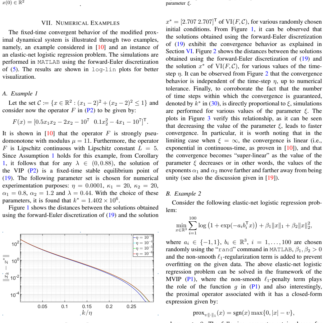
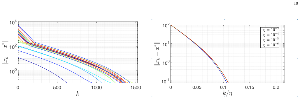
[Section VII-A, Fig. 2] The statement that convergence is "independent of the time-step eta up to numerical tolerance" is qualitative. Since the paper's discrete-time theory has a specific bound with eta*, it would be helpful to indicate how the observed thresholds compare with the theoretical prediction for the chosen eta values.
[Section VII-B, Example 2] The values mu = 0.5 and L = 0.5 for the logistic-regression operator are asserted without derivation. Please provide a short justification or a reference, since the admissible range lambda in (0, 2*mu/L^2) depends on these constants.

Circularity Check

1 steps flagged · score 4.0 of 10

Discrete-time fixed-step guarantee is imported from an unpublished co-authored preprint; continuous fixed-time result is self-contained.

self citation load bearing [Section VI, proof of Theorem 4; Corollary 2 (Eqs. (26), (30))]
"Furthermore, it can be verified that all the requirements as stated in [22, Theorem 4] are met. ... Hence, for every ǫ > 0 and every T ≥ 0, there exists η∗ > 0 with the following property: for any η ∈ (0, η∗] and a solution xk of (24) starting from the point x0, there exists a solution x of (20) starting from the point x0 such that the solutions x and xk are (T, ǫ)-close."

Equation (26) is obtained by substituting the exact trajectory bound (27) into the triangle inequality (28) using the '(T,ǫ)-close' property, and that property is not proved here: the proof states only that 'all the requirements as stated in [22, Theorem 4] are met.' Reference [22] is an unpublished arXiv preprint by Benosman, Romero, and Cherian, and Benosman is a co-author of the present paper. No independent derivation of the closeness estimate is given. Since the field in (5) is superlinear for α2 > 1, forward-Euler closeness over arbitrary initial conditions is not automatic, so the whole fixed-number-of-steps claim (Corollary 2, Eq. (30)) reduces to this load-bearing self-citation rather than to the paper's own analysis.

full rationale

The continuous-time part of the paper is self-contained: Theorem 1 derives the contraction property of the proximal operator directly from Assumption 1 and standard proximal inequalities; Theorem 2 obtains the fixed-time estimate (17) from Lemma 1, with no fitted parameters and no reliance on the authors' prior work. Lemma 4, Proposition 2, and Theorem 3 are also proved internally. The substantive circularity is confined to the discrete-time contribution: Theorem 4 and Corollary 2 delegate the decisive (T,ǫ)-closeness of Euler solutions to [22, Thm 4], an unpublished arXiv preprint including co-author Benosman. The paper verifies hypotheses but does not prove that theorem, so the fixed-number-of-steps bound (26)/(30) rests on a load-bearing self-citation. This does not undermine the continuous fixed-time stability claim, so the score is moderate rather than high.

Assumptions & free parameters 3 free parameters · 7 assumptions · 0 invented entities

The central continuous-time result rests on standard strong monotonicity/Lipschitz assumptions and standard proximal operator theory. The discretization result additionally imports an external consistency theorem from [22], a preprint by a co-author, which is not proved in the paper. The numerical examples introduce hand-chosen parameters and asserted constants μ and L that are not fully verified.

free parameters (3)

Gains κ1, κ2 and exponents α1, α2 = null (example choices: 20,20,0.8,1.2 and 20,200,0.97,1.03)
Design parameters of the modified flow. The fixed-time bound in Remark 6 decreases as κ grow, but the theorem requires no specific values. Chosen by hand, not fitted to data.
Step-size λ and discretization step η = null (example choices: λ=0.44 or 0.005, η=0.0001)
λ must lie in (0,2μ/L^2) and η must be below η* from Theorem 4. Chosen empirically for the examples.
Constants μ and L in Example 2 = μ=0.5, L=0.5
Asserted without verification. They define the allowed λ range (0,4); if actual values differ, the claim that Assumption 1 holds is unsupported.

assumptions (7)

domain assumption Assumption 1: F is strongly monotone with modulus μ and Lipschitz with constant L
Standing assumption for Theorem 1, Theorem 2, and Corollary 2.
standard math Existence and uniqueness of the MVIP solution under strong monotonicity and Lipschitz continuity (Noor [26, Theorem 3.1])
Used in Lemma 2 and Remark 5 to guarantee a unique equilibrium point for the nominal and modified dynamics.
standard math Proximal operator characterization and nonexpansiveness (Bauschke-Combettes [25, Prop. 12.26, 12.28])
Basis for Lemma 2 and for the Lipschitz continuity of the vector field in Theorem 2.
standard math Fixed-time stability Lyapunov criterion (Polyakov [14], Lemma 1)
Used to conclude fixed-time stability from the bound (17) in the proof of Theorem 2.
domain assumption Strong pseudomonotonicity suffices for contraction in the projection case (proof of [8, Theorem 2])
Supports Remark 7 and Corollary 1 for modified projected dynamics.
domain assumption (T,ε)-closeness theorem for discretization of differential inclusions ([22, Theorem 4])
Load-bearing for Theorem 4 and Corollary 2; not proved in this paper, only cited.
standard math Existence of Carathéodory solutions for upper semicontinuous set-valued maps (Filippov [33, Theorem 2.7.1])
Used in the proof of Theorem 3 to assert solution existence for differential inclusions.

how reviews work

0 comments

Cite this review

Pith. "Pith review of Fixed-Time Stable Proximal Dynamical System for Solving MVIPs." pith.science (2026). https://pith.science/paper/FMUK7CTW

@misc{pith2026190803517,
  author       = {Pith},
  title        = {Pith review of: Fixed-Time Stable Proximal Dynamical System for Solving MVIPs},
  year         = {2026},
  howpublished = {\url{https://pith.science/paper/FMUK7CTW}},
  note         = {Machine review of arXiv:1908.03517}
}

read the original abstract

In this paper, a novel modified proximal dynamical system is proposed to compute the solution of a mixed variational inequality problem (MVIP) within a fixed time, where the time of convergence is finite and is uniformly bounded for all initial conditions. Under the assumptions of strong monotonicity and Lipschitz continuity, it is shown that a solution of the modified proximal dynamical system exists, is uniquely determined, and converges to the unique solution of the associated MVIP within a fixed time. Furthermore, the fixed-time stability of the modified projected dynamical system continues to hold, even if the assumption of strong monotonicity is relaxed to that of strong pseudomonotonicity. Finally, it is shown that the solution obtained using the forward-Euler discretization of the proposed modified proximal dynamical system converges to an arbitrarily small neighborhood of the solution of the associated MVIP within a fixed number of time steps, independent of the initial conditions.

Figures

Figures reproduced from arXiv: 1908.03517 by the authors.

**Figure 1.** Example 1: Plots of kxk − x ∗k2 vs. k for various initial conditions x(0) ∈ R2 . VII. NUMERICAL EXAMPLES The fixed-time convergent behavior of the modified proximal dynamical system is illustrated through two examples, namely, an example considered in [10] and an instance of an elastic-net logistic regression problem. The simulations are performed in MATLAB using the forward-Euler discretization of (5). The results… view at source ↗

**Figure 2.** Example 1: Plots of kxk − x ∗k2 vs. k for various values of the time-step η. 500 1000 1500 2000 2500 3000 3500 10-4 10-2 100 [PITH_FULL_IMAGE:figures/full_fig_p009_2.png] view at source ↗

**Figure 4.** Example 2: Plots of kxk − x ∗k2 vs. k for various initial conditions x(0) ∈ R3 . η = 0.0001, κ1 = 20, κ2 = 200, α1 = 0.97, α2 = 1.03 and λ = 0.005. It can be verified that Assumption 1 also holds for this example (with µ = 0.5 and L = 0.5) and hence, from Theorem 2, it follows that for any λ ∈ (0, 4), the solution of the MVIP (P1) is a fixed-time stable equilibrium point of (5) [PITH_FULL_IMAGE:figures/full_fig_p01… view at source ↗

Discussion (0). Continue with ORCID to comment.

Reference graph

Works this paper leans on

42 extracted references · 41 canonical work pages

[22]

Optimizing dee p neural networks via discretization of ﬁnite-time convergent ﬂows ,

M. Benosman, O. Romero, and A. Cherian, “Optimizing dee p neural networks via discretization of ﬁnite-time convergent ﬂows ,” 2020, arXiv e-Print

work page 2020
[8]

On the global exponential stability of a projected dynamical system for strongly pseu domonotone variational inequalities,

N. T. T. Ha, J.-J. Strodiot, and P . T. Vuong, “On the global exponential stability of a projected dynamical system for strongly pseu domonotone variational inequalities,” Optimization Letters, vol. 12, no. 7, pp. 1625– 1638, 2018

work page 2018
[1]

Facchinei and J.-S

F. Facchinei and J.-S. Pang, Finite-Dimensional Variational Inequalities and Complementarity Problems . Springer, 2003

work page 2003
[2]

Giannessi, A

F. Giannessi, A. Maugeri, and P . M. Pardalos, Equilibrium Problems: Nonsmooth Optimization and Variational Inequality Models . Springer, 2001

work page 2001
[3]

Nas h equilibria, variational inequalities, and dynamical systems,

E. Cavazzuti, M. Pappalardo, and M. Passacantando, “Nas h equilibria, variational inequalities, and dynamical systems,” Journal of Optimiza- tion Theory and Applications , vol. 114, no. 3, pp. 491–506, 2002

work page 2002
[4]

Convex optimization, game theory, and variational inequality the ory,

G. Scutari, D. P . Palomar, F. Facchinei, and J.-S. Pang, “ Convex optimization, game theory, and variational inequality the ory,” IEEE Signal Processing Magazine , vol. 27, no. 3, pp. 35–49, 2010

work page 2010
[5]

Approxim ating optimal control problems governed by variational inequalities,

V . Barbu, P . Neittaanm¨ aki, and A. Niemist¨ o, “Approxim ating optimal control problems governed by variational inequalities,” Numerical Func- tional Analysis and Optimization , vol. 15, no. 5-6, pp. 489–502, 1994

work page 1994
[6]

A variational inequality approach to con- strained control problems for parabolic equations,

P . Neittaanm¨ aki and D. Tiba, “A variational inequality approach to con- strained control problems for parabolic equations,” Applied Mathematics and Optimization , vol. 17, no. 1, pp. 185–201, 1988

work page 1988

Show all 42 references

[7]

Kinderlehrer and G

D. Kinderlehrer and G. Stampacchia, An Introduction to Variational Inequalities and Their Applications . SIAM, 2000

2000
[9]

Proximal gra dient ﬂow and Douglas–Rachford splitting dynamics: Global exponent ial stability via integral quadratic constraints,

S. Hassan-Moghaddam and M. R. Jovanovi´ c, “Proximal gra dient ﬂow and Douglas–Rachford splitting dynamics: Global exponent ial stability via integral quadratic constraints,” Automatica, vol. 123, 2021, article 109311

2021
[10]

Solving pseudomonotone variational inequalities and pseudoconvex optimization problems using the projecti on neural network,

X. Hu and J. Wang, “Solving pseudomonotone variational inequalities and pseudoconvex optimization problems using the projecti on neural network,” IEEE Transactions on Neural Networks , vol. 17, no. 6, pp. 1487–1499, 2006

2006
[11]

A general methodology for designing globally convergent optimization neural networks,

Y . Xia and J. Wang, “A general methodology for designing globally convergent optimization neural networks,” IEEE Transactions on Neural Networks, vol. 9, no. 6, pp. 1331–1343, 1998

1998
[12]

A projection neural netwo rk and its application to constrained optimization problems,

Y . Xia, H. Leung, and J. Wang, “A projection neural netwo rk and its application to constrained optimization problems,” IEEE Transactions on Circuits and Systems I: Fundamental Theory and Application s, vol. 49, no. 4, pp. 447–458, 2002

2002
[13]

Finite-Time stability o f continuous autonomous systems,

S. P . Bhat and D. S. Bernstein, “Finite-Time stability o f continuous autonomous systems,” SIAM Journal on Control and Optimization , vol. 38, no. 3, pp. 751–766, 2000

2000
[14]

Nonlinear feedback design for fixed-tim e stabilization of linear control systems,

A. Polyakov, “Nonlinear feedback design for fixed-tim e stabilization of linear control systems,” IEEE Transactions on Automatic Control , vol. 57, no. 8, pp. 2106–2110, 2012

2012
[15]

Finite-Tim e and ﬁxed- time stabilization: Implicit Lyapunov function approach,

A. Polyakov, D. Eﬁmov, and W. Perruquetti, “Finite-Tim e and ﬁxed- time stabilization: Implicit Lyapunov function approach, ” Automatica, vol. 51, pp. 332–340, 2015

2015
[16]

Finite-Time convergent gradient flows wi th applications to network consensus,

J. Cort´ es, “Finite-Time convergent gradient flows wi th applications to network consensus,” Automatica, vol. 42, no. 11, pp. 1993–2000, 2006

1993
[17]

Convex optimization via finite-tim e projected gradient flows,

F. Chen and W. Ren, “Convex optimization via finite-tim e projected gradient flows,” in Proceedings of the Conference on Decision and Control. IEEE, 2018, pp. 4072–4077

2018
[18]

A fixed time distribute d opti- mization: A sliding mode perspective,

C. Li, X. Y u, X. Zhou, and W. Ren, “A fixed time distribute d opti- mization: A sliding mode perspective,” in Proceedings of the Annual 11 Conference of the Industrial Electronics Society . IEEE, 2017, pp. 8201– 8207

2017
[19]

Fixed-Time stable gradient ﬂow s: Applica- tions to continuous-time optimization,

K. Garg and D. Panagou, “Fixed-Time stable gradient ﬂow s: Applica- tions to continuous-time optimization,” IEEE Transactions on Automatic Control, vol. 66, no. 5, pp. 2002–2015, 2021

2002
[20]

Finite-Time convergence in continuous- time optimization,

O. Romero and M. Benosman, “Finite-Time convergence in continuous- time optimization,” in Proceedings of the International Conference on Machine Learning , 2020, pp. 8200–8209

2020
[21]

Time-Varying continuous-time optimisation with pre-deﬁned ﬁnite-time stability,

——, “Time-Varying continuous-time optimisation with pre-deﬁned ﬁnite-time stability,” International Journal of Control , pp. 1–18, 2020

2020
[23]

On the maximal monotonicity of subd ifferential mappings,

R. T. Rockafellar, “On the maximal monotonicity of subd ifferential mappings,” Paciﬁc Journal of Mathematics , vol. 33, no. 1, pp. 209–216, 1970

1970
[24]

Seven kinds of monoton e maps,

S. Karamardian and S. Schaible, “Seven kinds of monoton e maps,” Journal of Optimization Theory and Applications , vol. 66, no. 1, pp. 37–46, 1990

1990
[25]

H. H. Bauschke and P . L. Combettes, Convex Analysis and Monotone Operator Theory in Hilbert Spaces . Springer, 2017

2017
[26]

Mixed variational inequalities,

M. Aslam Noor, “Mixed variational inequalities,” Applied Mathematics Letters, vol. 3, no. 2, pp. 73–75, 1990

1990
[27]

Qualitative properties of s trongly pseudomonotone variational inequalities,

P . T. Vuong and P . D. Khanh, “Qualitative properties of s trongly pseudomonotone variational inequalities,” Optimization Letters, vol. 10, no. 8, pp. 1669–1679, 2016

2016
[28]

On general mixed variational inequalities,

M. Aslam Noor, K. Inayat Noor, and H. Y aqoob, “On general mixed variational inequalities,” Acta Applicandae Mathematicae , vol. 110, no. 1, pp. 227–246, 2010

2010
[29]

Theory of variational inequa lities with applications to problems of ﬂow through porous media,

J. T. Oden and N. Kikuchi, “Theory of variational inequa lities with applications to problems of ﬂow through porous media,” International Journal of Engineering Science , vol. 18, no. 10, pp. 1173–1284, 1980

1980
[30]

Consistent di scretization of finite-time and fixed-time stable systems,

A. Polyakov, D. Eﬁmov, and B. Brogliato, “Consistent di scretization of finite-time and fixed-time stable systems,” SIAM Journal on Control and Optimization, vol. 57, no. 1, pp. 78–103, 2019

2019
[31]

Dynamical properties of hybrid systems simulators,

R. G. Sanfelice and A. R. Teel, “Dynamical properties of hybrid systems simulators,” Automatica, vol. 46, no. 2, pp. 239–248, 2010

2010
[32]

Stability and stabiliz ation of discontin- uous systems and nonsmooth Lyapunov functions,

A. Bacciotti and F. Ceragioli, “Stability and stabiliz ation of discontin- uous systems and nonsmooth Lyapunov functions,” ESAIM: Control, Optimisation and Calculus of V ariations , vol. 4, pp. 361–376, 1999

1999
[33]

A. F. Filippov, Differential Equations with Discontinuous Righthand Sides. Springer, 1988

1988
[34]

Finite- Time stability for differential inclusions with applicati ons to neural networks,

R. Matusik, A. Nowakowski, S. Plaskacz, and A. Rogowski , “Finite- Time stability for differential inclusions with applicati ons to neural networks,” SIAM Journal on Control and Optimization , vol. 58, no. 5, pp. 2854–2870, 2020

2020
[35]

A forward-backward dynami cal approach to the minimization of the sum of a nonsmooth convex with a smo oth nonconvex function,

R. I. Bot ¸ and E. R. Csetnek, “A forward-backward dynami cal approach to the minimization of the sum of a nonsmooth convex with a smo oth nonconvex function,” ESAIM: Control, Optimisation and Calculus of V ariations, vol. 24, no. 2, pp. 463–477, 2018

2018
[36]

J. K. Hale, Ordinary Differential Equations . Krieger Publishing Company, 1980

1980
[37]

On a class of complete poly nomial vector fields in the plane,

C. Chicone and J. Sotomayor, “On a class of complete poly nomial vector fields in the plane,” Journal of Differential Equations , vol. 61, no. 3, pp. 398–418, 1986

1986
[38]

Chicone, Ordinary Differential Equations with Applications

C. Chicone, Ordinary Differential Equations with Applications . Springer, 2006

2006
[39]

H. K. Khalil, Nonlinear Systems . Prentice Hall, 2002

2002
[40]

R. P . Agarwal and V . Lakshmikantham, Uniqueness and Nonuniqueness Criteria for Ordinary Differential Equations . World Scientiﬁc Publish- ing Company, 1993. APPENDIX A PROOF OF THEOREM 1 Proof. For any given x ∈ Rn, from [ 25, Proposition 12.26], it follows that ⟨y(x) − (x −...

1993
[41]

(37) Using ( 35) and ( 37), the right hand side of ( 34) can be upper bounded as follows: ⟨x − y(x), x∗ − y(x)⟩ ≤ −λµ‖x∗ − y(x)‖2 + 1 2 ‖x − y(x)‖2 + λ2L2 2 ‖x∗ − y(x)‖2

can further be upper bounded as follows: λL‖x−y(x)‖‖x∗−y(x)‖ ≤ 1 2 ‖x−y(x)‖2+ λ2L2 2 ‖x∗−y(x)‖2 and so, ( 36) results into: λ ⟨F (y(x)) − F (x), y(x) − x∗⟩ ≤ λ2L2 2 ‖x∗ − y(x)‖2 + 1 2 ‖x − y(x)‖2. (37) Using ( 35) and ( 37), the right hand side of ( 34) can be upper bounded as...
[42]

is also a solution corresponding to the vector ﬁeld X, under the reparameterization of time given in ( 42). Furthermore, by following the steps, similar to the ones given in the proof of the ﬁrst claim and recalling that the vector ﬁeld X is locally Lipschitz continuous on Rn,...

Pith tools

Reviewed August 14, 2026 · model on record in the stance chip above.

[1] [22]

Optimizing dee p neural networks via discretization of ﬁnite-time convergent ﬂows ,

M. Benosman, O. Romero, and A. Cherian, “Optimizing dee p neural networks via discretization of ﬁnite-time convergent ﬂows ,” 2020, arXiv e-Print

work page 2020

[2] [8]

On the global exponential stability of a projected dynamical system for strongly pseu domonotone variational inequalities,

N. T. T. Ha, J.-J. Strodiot, and P . T. Vuong, “On the global exponential stability of a projected dynamical system for strongly pseu domonotone variational inequalities,” Optimization Letters, vol. 12, no. 7, pp. 1625– 1638, 2018

work page 2018

[3] [1]

Facchinei and J.-S

F. Facchinei and J.-S. Pang, Finite-Dimensional Variational Inequalities and Complementarity Problems . Springer, 2003

work page 2003

[4] [2]

Giannessi, A

F. Giannessi, A. Maugeri, and P . M. Pardalos, Equilibrium Problems: Nonsmooth Optimization and Variational Inequality Models . Springer, 2001

work page 2001

[5] [3]

Nas h equilibria, variational inequalities, and dynamical systems,

E. Cavazzuti, M. Pappalardo, and M. Passacantando, “Nas h equilibria, variational inequalities, and dynamical systems,” Journal of Optimiza- tion Theory and Applications , vol. 114, no. 3, pp. 491–506, 2002

work page 2002

[6] [4]

Convex optimization, game theory, and variational inequality the ory,

G. Scutari, D. P . Palomar, F. Facchinei, and J.-S. Pang, “ Convex optimization, game theory, and variational inequality the ory,” IEEE Signal Processing Magazine , vol. 27, no. 3, pp. 35–49, 2010

work page 2010

[7] [5]

Approxim ating optimal control problems governed by variational inequalities,

V . Barbu, P . Neittaanm¨ aki, and A. Niemist¨ o, “Approxim ating optimal control problems governed by variational inequalities,” Numerical Func- tional Analysis and Optimization , vol. 15, no. 5-6, pp. 489–502, 1994

work page 1994

[8] [6]

A variational inequality approach to con- strained control problems for parabolic equations,

P . Neittaanm¨ aki and D. Tiba, “A variational inequality approach to con- strained control problems for parabolic equations,” Applied Mathematics and Optimization , vol. 17, no. 1, pp. 185–201, 1988

work page 1988