pith. sign in

arxiv: 2605.21564 · v2 · pith:FNQ6K2IBnew · submitted 2026-05-20 · 🌀 gr-qc

Astrophysical Objects in Modified Theories of Gravity

Pith reviewed 2026-05-22 09:37 UTC · model grok-4.3

classification 🌀 gr-qc
keywords modified gravitycompact starsneutron starsstrange starsf(Q) gravityf(T) gravitygravitational decouplingMIT Bag equation of state
0
0 comments X

The pith

Modified gravity models of compact stars change their maximum mass, radius and stability while matching observations.

A machine-rendered reading of the paper's core claim, the machinery that carries it, and where it could break.

The paper builds exact solutions for charged neutron stars in f(Q) gravity and anisotropic strange stars in f(T) gravity. It employs conformal symmetry together with the MIT Bag equation of state for the first family and minimal or complete geometric deformation for the second. Physical viability is checked with energy conditions, the generalized Tolman-Oppenheimer-Volkoff equation, causality, and Herrera's cracking criterion. A Bayesian analysis then constrains the free parameters against NICER mass-radius data. The central result is that the extra gravitational degrees of freedom can shift stellar properties without breaking observational compatibility.

Core claim

Exact analytic interior solutions for compact stars are obtained in f(Q) gravity by imposing conformal symmetry and the MIT Bag equation of state, then matched to the Bardeen exterior; in f(T) gravity the same stars are generated by minimal and complete geometric deformation that adds extra sources while preserving regularity and vanishing complexity. When these families are confronted with energy conditions, stability criteria and NICER observations, the modified-gravity parameters are shown to alter maximum mass, radius and stability ranges while remaining consistent with the data.

What carries the argument

Conformal symmetry plus the MIT Bag equation of state for isotropic charged models in f(Q) gravity, together with minimal and complete geometric deformation for anisotropic models in f(T) gravity.

If this is right

  • Varying the modified-gravity parameters shifts the maximum mass and radius of the star models.
  • Stability against cracking holds inside restricted intervals of those parameters.
  • Bayesian inference using NICER data yields finite posterior ranges for the extra gravitational parameters.
  • The models continue to satisfy the null, weak, strong and dominant energy conditions.
  • Additional matter sources such as dark-matter components can be introduced through the geometric-deformation sector.

Where Pith is reading between the lines

These are editorial extensions of the paper, not claims the author makes directly.

  • Future higher-precision mass-radius data could exclude entire intervals of the modified-gravity parameter space.
  • The same deformation techniques could be applied to rotating or magnetized stars to test whether the stability conclusions persist.
  • If the Bayesian preference for non-zero modified-gravity parameters survives larger data sets, it would motivate analogous studies of white dwarfs or black-hole shadows.

Load-bearing premise

The MIT Bag equation of state together with conformal symmetry supplies a realistic description of the stellar interior that can be joined to the Bardeen exterior without unphysical surface layers or violated junction conditions.

What would settle it

A precise mass-radius measurement of a compact star that lies outside every allowed curve produced by the f(Q) and f(T) families for any parameter values still consistent with the energy conditions and stability tests.

Figures

Figures reproduced from arXiv: 2605.21564 by Sneha Pradhan.

Figure 1.1
Figure 1.1. Figure 1.1: Hertzsprung–Russell (HR) diagram displaying stellar luminosity against spectral type for approximately four million stars within 5000 light-years of the Sun. The main sequence (diagonal band), red giant branch, horizontal branch, and white dwarf region are clearly visible, representing different stages of stellar evolution.Credit: ESA/Gaia/DPAC [5]. However, as the nuclear fuel in the stellar core is gra… view at source ↗
Figure 1.2
Figure 1.2. Figure 1.2: First detect image of the supermassive black hole located at the center of the M87 galaxy. (Image credit: EHT Collaboration, 2019). The X-ray source Cygnus X-1, recognized as the first confirmed candidate for a stellar￾mass black hole, was independently discovered by Bolton [42] and Webster & Murdin [43]. Subsequent astronomical studies provided further evidence for the existence of stellar-mass black ho… view at source ↗
Figure 1.3
Figure 1.3. Figure 1.3: Moving a vector around a closed loop changes its direction, measured by Rν βαµ. In the framework of GR, the curvature tensor arises solely from the Levi-Civita connection, which is symmetric and metric-compatible. This ensures that torsion and non-metricity vanish, and curvature fully encodes the gravitational interaction. However, in more general geometric theories such as those incorporating torsion or… view at source ↗
Figure 1.4
Figure 1.4. Figure 1.4: Left panel: In Euclidean geometry, parallel transport along two vectors forms a closed parallelogram. Right panel: In a space with torsion, the parallelogram does not close; the separation between the endpoints measures the torsion tensor T α µν. Thus, The torsion tensor has an interesting geometrical interpretation: if one builds infinitesimal parallelograms in the manifold (by parallel transport), the … view at source ↗
Figure 1.5
Figure 1.5. Figure 1.5: Change in the length of a vector under parallel transport arises from non-metricity. However, in a non-metric geometry condition ∇λgµν ̸= 0 holds. In this case, the connection allows the metric itself to vary from point to point under parallel transport. Physically, this means that as a vector is carried along a path from one point p to another point q, its length or magnitude can change. From Fig. (1.5)… view at source ↗
Figure 1.6
Figure 1.6. Figure 1.6: The rotation of a vector transported along a closed curve given by Rα βµν. In contrast, the symmetric part Rα (β)µν arises in non-metric geometries and describes a change in the magnitude (length) of the vector after parallel transport. Hence, in a general affine geometry, curvature can induce both a rotational and a stretching effect on transported vectors. Fig. (1.6) illustrates the rotation of a vecto… view at source ↗
Figure 1.7
Figure 1.7. Figure 1.7: Schematic classification of higher-order gravity theories obtained by incorporating additional curvature invariants into the Lagrangian of GR. Higher-order field equations: Although Einstein’s field equations contain derivatives only up to the second order, several modified gravity theories extend this idea by including higher-order derivatives. Although such extensions often introduce mathematical compl… view at source ↗
Figure 1.8
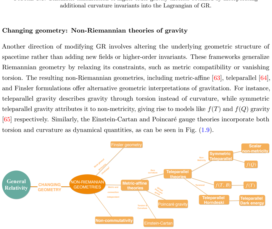
Figure 1.8. Figure 1.8: Schematic classification of higher-order gravity theories obtained by incorporating additional curvature invariants into the Lagrangian of GR. Changing geometry: Non-Riemannian theories of gravity Another direction of modifying GR involves altering the underlying geometric structure of spacetime rather than adding new fields or higher-order invariants. These frameworks generalize Riemannian geometry by r… view at source ↗
Figure 1.9
Figure 1.9. Figure 1.9: Schematic classification of higher-order gravity theories obtained by incorporating additional curvature invariants into the Lagrangian of GR [PITH_FULL_IMAGE:figures/full_fig_p040_1_9.png] view at source ↗
Figure 1.10
Figure 1.10. Figure 1.10: A schematic diagram among the relation of energy condition: An arrow from A to B in the illustration indicates that A implies B. The NEC requires the energy density measured by any null observer to be non-negative. It serves as a foundational requirement upon which both the WEC and the SEC are built. Formally, for any null vector l m, Tmn l ml n ≥ 0, which translates to the effective inequalities ρ + pr… view at source ↗
Figure 2.1
Figure 2.1. Figure 2.1: , we observe that model-I exhibits finite, continuous, and monotonically increasing metric functions throughout the star. In contrast, model-II develops a central singularity owing to the linear choice of the conformal factor, although the metric potentials remain well behaved away from the core. This indicates that the power-law conformal factor is more suitable for constructing physically viable compac… view at source ↗
Figure 2.2
Figure 2.2. Figure 2.2: , both the pressure and energy density attain their maximum values at the stellar center and decrease smoothly towards the surface, where the pressure vanishes. This behavior confirms the physical acceptability of the constructed models, with the concave nature of the profiles arising from the combined effects of conformal symmetry and electric charge. PSR J1614-2230 PSR J1903+327 Vela X-1 Cen X-3 SMC X-… view at source ↗
Figure 2.3
Figure 2.3. Figure 2.3: Behavior of pressure gradient and matter density gradient for model-I (upper panel) and model-II (lower panel). Here, we consider m = −2, n = 0.02 for model-I and m = 2, n = −1 for model-II. 3. Energy conditions: Energy conditions provide essential consistency checks for physically realistic stellar models and have been extensively discussed earlier. In the present analysis, we verify the null, weak, str… view at source ↗
Figure 2.4
Figure 2.4. Figure 2.4: Behavior of energy conditions for model-I (upper panel) and model-II (lower panel). Here, we consider m = −2, n = 0.02 for model-I and m = 2, n = −1 for model-II. 2. Relativistic adiabatic index: The relativistic adiabatic index provides an important criterion for assessing the dynamical stability of compact stars. As discussed earlier, stability requires Γ > 4/3. From [PITH_FULL_IMAGE:figures/full_fig_… view at source ↗
Figure 2.5
Figure 2.5. Figure 2.5: Behavior of adiabatic index for model-I (left panel) and model-II (right panel). Here, we consider m = −2, n = 0.02 for model-I and m = 2, n = −1 for model-II. 3. Equilibrium conditions: The equilibrium of a charged compact star is governed by the TOV equation, which ensures the balance between gravitational, hydrostatic, and electric [PITH_FULL_IMAGE:figures/full_fig_p067_2_5.png] view at source ↗
Figure 2.6
Figure 2.6. Figure 2.6: Behavior of different forces for model-I (left panel) and model-II (right panel). The different colors represents, PSR J1614-2230(⋆), PSR J1903+327 (⋆), Vela X-1 (⋆), Cen X-3 (⋆), and SMC X-1 (⋆). Here, we consider m = −2, n = 0.02 for model-I and m = 2, n = −1 for model-II. forces. For a static and spherically symmetric configuration, these forces are given by Fg = − ν ′ 2 (ρ eff + p eff), Fh = − dpeff … view at source ↗
Figure 2.7
Figure 2.7. Figure 2.7: Comparison between the Bardeen and R-N spacetime. 2.7 Conclusion In this chapter, we explored the structure of charged compact stars within the framework of f(Q) gravity by employing CKVs. The stellar interior is modeled as a charged perfect fluid obeying [PITH_FULL_IMAGE:figures/full_fig_p070_2_7.png] view at source ↗
Figure 3.1
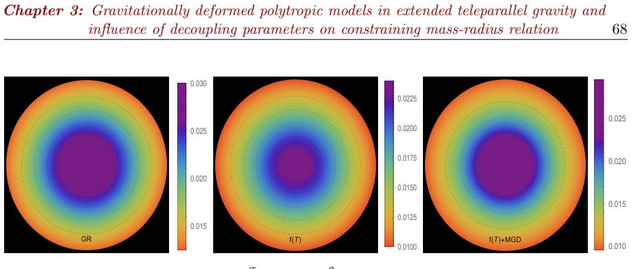
Figure 3.1. Figure 3.1: The density profile [ρ eff(r)] in [km−2 ] along to the radial distance r of the stellar model for solution 3.3.1 [Θ0 0 = ρ] in context of GR α = 0.0, ζ1 = 1.0, ζ2 = 0.0 [km−2 ]  -left panel, f(T) [PITH_FULL_IMAGE:figures/full_fig_p083_3_1.png] view at source ↗
Figure 3.2
Figure 3.2. Figure 3.2: The radial pressure profile [p eff r (r)] in [km−2 ] along to the radial distance r of the stellar model for solution 3.3.1 [Θ0 0 = ρ] in context of GR α = 0.0, ζ1 = 1.0, ζ2 = 0.0 [km−2 ]  -left panel, f(T) [PITH_FULL_IMAGE:figures/full_fig_p083_3_2.png] view at source ↗
Figure 3.3
Figure 3.3. Figure 3.3: The effective tangential pressure profile [p eff t (r)] in [km−2 ] along to the radial distance r of the stellar model for solution 3.3.1 [Θ0 0 = ρ] in context of GR α = 0.0, ζ1 = 1.0, ζ2 = 0.0 [km−2 ]  -left panel, f(T) [PITH_FULL_IMAGE:figures/full_fig_p083_3_3.png] view at source ↗
Figure 3.4
Figure 3.4. Figure 3.4: The effective anisotropy profile [∆eff(r)] in [km−2 ] along to the radial distance r of the stellar model for solution 3.3.1 [Θ0 0 = ρ] in context of GR α = 0.0, ζ1 = 1.0, ζ2 = 0.0 [km−2 ]  -left panel, f(T) [PITH_FULL_IMAGE:figures/full_fig_p084_3_4.png] view at source ↗
Figure 3.5
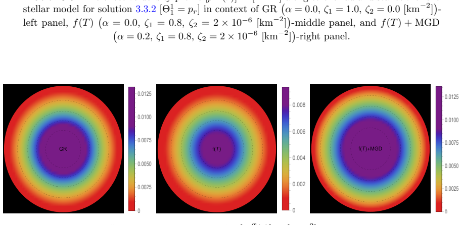
Figure 3.5. Figure 3.5: The effective density profile [ρ eff(r)] in [km−2 ] along to the radial distance r of the stellar model for solution 3.3.2 [Θ1 1 = pr] in context of GR α = 0.0, ζ1 = 1.0, ζ2 = 0.0 [km−2 ]  - left panel, f(T) [PITH_FULL_IMAGE:figures/full_fig_p084_3_5.png] view at source ↗
Figure 3.6
Figure 3.6. Figure 3.6: The effective radial pressure profile [p eff r (r)] in [km−2 ] along to the radial distance r of the stellar model for solution 3.3.2 [Θ1 1 = pr] in context of GR α = 0.0, ζ1 = 1.0, ζ2 = 0.0 [km−2 ]  -left panel, f(T) [PITH_FULL_IMAGE:figures/full_fig_p084_3_6.png] view at source ↗
Figure 3.7
Figure 3.7. Figure 3.7: The effective tangential pressure profile [p eff t (r)] in [km−2 ] along to the radial distance r of the stellar model for solution 3.3.2 [Θ1 1 = pr] in context of GR α = 0.0, ζ1 = 1.0, ζ2 = 0.0 [km−2 ]  -left panel, f(T) [PITH_FULL_IMAGE:figures/full_fig_p085_3_7.png] view at source ↗
Figure 3.8
Figure 3.8. Figure 3.8: The effective anisotropy profile [∆eff(r)] in [km−2 ] along to the radial distance r of the stellar model for solution 3.3.2 [Θ1 1 = pr] in context of GR α = 0.0, ζ1 = 1.0, ζ2 = 0.0 [km−2 ]  -left panel, f(T) [PITH_FULL_IMAGE:figures/full_fig_p085_3_8.png] view at source ↗
Figure 3.9
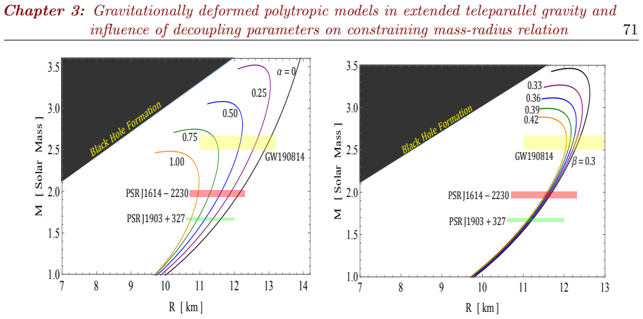
Figure 3.9. Figure 3.9: The M − R curves for different free parameters values α-left panel with fixed β = 0.33, γ = 20, ζ1 = 0.5 and right figure shows the M − R curves for different β with fixed α = 0.5, γ = 15, and ζ1 = 0.5. The both figures represent the mass-radius relation for solution 3.3.1 Θ0 0 = ρ [PITH_FULL_IMAGE:figures/full_fig_p086_3_9.png] view at source ↗
Figure 3.10
Figure 3.10. Figure 3.10: The M − R curves for different free parameters values γ-left panel with fixed β = 0.33, α = 0.5 km2 , ζ1 = 0.5 and right figure shows the M − R curves for different ζ1 with fixed α = 0.5, γ = 15, and β = 0.33. The both figures represent the mass-radius relation for solution 3.3.1 Θ0 0 = ρ [PITH_FULL_IMAGE:figures/full_fig_p086_3_10.png] view at source ↗
Figure 3.11
Figure 3.11. Figure 3.11: The M − R curves for different free parameters values α-left panel with fixed β = 0.33, γ = 20, ζ1 = 0.3 and right figure shows the M − R curves for different ζ1 with fixed α = 0.2, γ = 20, and β = 0.33. The both figures represent the mass-radius relation for solution 3.3.2 Θ1 1 = pr [PITH_FULL_IMAGE:figures/full_fig_p087_3_11.png] view at source ↗
Figure 3.12
Figure 3.12. Figure 3.12: Graphical analysis of adiabatic index for different values of the model parameter ζ1 for the solution ρ = Θ0 0 and pr = Θ1 1 respectively, where α = 0.5 km2 and α = 0.2 km2 respectively [PITH_FULL_IMAGE:figures/full_fig_p088_3_12.png] view at source ↗
Figure 3.13
Figure 3.13. Figure 3.13: Graphical analysis of mass and dM dρc with respect to central density (ρc) for different values of the model parameter for the solution ρ = Θ0 0 . ζ1 = 0.60 ζ1 = 0.65 δζ1 = 0.01 pr = θ1 1 0.005 0.006 0.007 0.008 0.009 0.010 1.6 1.8 2.0 2.2 2.4 2.6 2.8 Central density (ρc) [km-2 ] Mass [M⊙] pr = θ1 1 ζ1 = 0.65 ζ1 = 0.60 δζ1 = 0.01 0.005 0.006 0.007 0.008 0.009 0.010 200 220 240 260 280 Central density (ρ… view at source ↗
Figure 3.14
Figure 3.14. Figure 3.14: Graphical analysis of mass and dM dρc w.r.t. central density (ρc) for different values of the model parameter for the solution pr = Θ1 1 . In this context, we analyze the stability of the solution ρ = Θ0 0 and pr = Θ1 1 in [PITH_FULL_IMAGE:figures/full_fig_p089_3_14.png] view at source ↗
Figure 4.1
Figure 4.1. Figure 4.1: Graphical analysis of energy density (left) [α = 0.1(⋆), α = 0.2(⋆), α = 0.3(⋆), α = 0.4(⋆), α = 0.5(⋆), α = 0.6(⋆)] and radial pressure (right) for C = 0.288 km−2 ; D = 0.1; A = 0.009 km−2 ; B = 0.000009 km−4 ;L = 0.0009 km−2 ; N = 0.0009 km−2 . model within the CGD framework of teleparallel gravity. The construction of a physically acceptable dark star model within the CGD framework requires a smooth m… view at source ↗
Figure 4.2
Figure 4.2. Figure 4.2: Graphical analysis of tangential pressure (left) and anisotropy (right) for C = 0.288 km−2 ; D = 0.1; A = 0.009 km−2 ; B = 0.000009 km−4 ;L = 0.0009 km−2 ; N = 0.0009 km−2 . ρ tot , p tot r , p tot t and anisotropy (∆tot) in Figs. 4.1 and 4.2 provides a comprehensive view of the energy distribution within the stellar model. Our analysis reveals that ρ tot , p tot r , and p tot t satisfy the essential cri… view at source ↗
Figure 4.3
Figure 4.3. Figure 4.3: Graphical analysis of the density gradient (left), the radial pressure gradient (middle) and the tangential pressure gradient (right) with respect to ’r,’ for C = 0.288 km−2 ; D = 0.1; A = 0.009 km−2 ; B = 0.000009 km−4 ;L = 0.0009 km−2 ; N = 0.0009 km−2 . From Figs. 4.1 and 4.2, it is evident that all energy conditions are satisfied throughout the stellar interior. The effective energy density remains p… view at source ↗
Figure 4.4
Figure 4.4. Figure 4.4: Stability analysis via adiabatic index (Γ) for C = 0.288 km−2 ; D = 0.1; A = 0.009 km−2 ; B = 0.000009 km−4 ;L = 0.0009 km−2 ; N = 0.0009 km−2 . α=0.1 α=0.2 α=0.3 α=0.4 α=0.5 α=0.6 0 2 4 6 8 0.0 0.2 0.4 0.6 0.8 1.0 r [km] Vr 2 α=0.1 α=0.2 α=0.3 α=0.4 α=0.5 α=0.6 0 2 4 6 8 0.0 0.2 0.4 0.6 0.8 1.0 1.2 r [km] Vt 2 α=0.1 α=0.2 α=0.3 α=0.4 α=0.5 α=0.6 0 2 4 6 8 0.00 0.05 0.10 0.15 r [km] |Vr 2 - Vt 2 | [PITH… view at source ↗
Figure 4.5
Figure 4.5. Figure 4.5: Stability analysis via speed of sound w.r.t. ’r’ for C = 0.288 km−2 ; D = 0.1; A = 0.009 km−2 ; B = 0.000009 km−4 ;L = 0.0009 km−2 ; N = 0.0009 km−2 . Smaller values of α are sufficient to maintain core stability, whereas near the stellar surface the influence of α becomes negligible, as the stability condition is satisfied throughout. 4.5.2 Causality criterion & Herrera’s cracking method The stability o… view at source ↗
Figure 4.6
Figure 4.6. Figure 4.6: Graphical analysis of mass (M⊙) with respect to central density ρc for C = 0.288 km−2 ; D = 0.1; A = 0.009 km−2 ; B = 0.000009 km−4 ;L = 0.0009 km−2 ; N = 0.0009 km−2 . 4.5.3 Harrison–Zeldovich–Novikov criterion The stability of the anisotropic dark star model is further examined using the HZN criterion, which is based on the response of the stellar mass to variations in the central density. According to… view at source ↗
Figure 4.7
Figure 4.7. Figure 4.7: Prediction of radii of some well-known compact objects from our model for different values of the decoupling parameter α (left) and model parameter ζ1 (right) [PITH_FULL_IMAGE:figures/full_fig_p100_4_7.png] view at source ↗
Figure 4.8
Figure 4.8. Figure 4.8: (Left panel) Equi-mass contour in ζ1 − ζ2 plane, (middle panel) in ζ1 − α plane, and (right panel) in ζ2 − α plane are shown. 4.7 Mass measurement via equi-mass planes In this section, a couple of contour plots are drawn for in-depth analysis of the mass of our current model. We have displayed the equi-mass contours in the ζ1 − ζ2 and ζ1 − α planes in the left and middle panels, respectively, of [PITH_F… view at source ↗
Figure 4.9
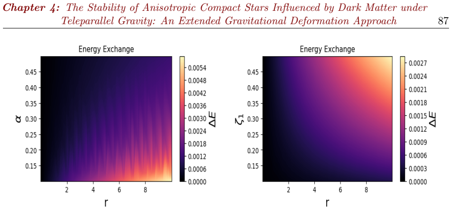
Figure 4.9. Figure 4.9: Energy exchange between the fluid and dark matter in the r − α plane (left) and r − ζ1 plane (right) for C = 0.288 km−2 ; D = 0.1; A = 0.009 km−2 ; B = 0.000009 km−4 ;L = 0.0009 km−2 ; N = 0.0009 km−2 . [170, 180], the energy exchanged between the two sources is quantified by the scalar δE, defined as δE = Φ ′ (r) 2 (ρ + pr), (4.27) where Φ(r) is the temporal deformation function. Since the energy densit… view at source ↗
Figure 5.1
Figure 5.1. Figure 5.1: The energy density (ε) (in MeV fm−3 )(left panel), pressure (p) (in MeV.fm−3 ) (middle panel), and speed of sound (c 2 s ) (in c 2 ) (right panel) as a function of baryon density (ρ) (in fm−3 ) for DDME2 [PITH_FULL_IMAGE:figures/full_fig_p111_5_1.png] view at source ↗
Figure 5.2
Figure 5.2. Figure 5.2: The marginalized posterior distributions of the f(Q) model parameters, obtained through Bayesian inference, for linear (red), logarithmic (purple), and exponential (green) models. The vertical lines indicate the 68% confidence interval of the parameters. The confidence ellipses for two-dimensional posterior distributions are plotted with 1σ, 2σ and 3σ confidence intervals. only moderately constrained, su… view at source ↗
Figure 5.3
Figure 5.3. Figure 5.3: Corner plots for the marginalized posterior distributions of the tidal deformability Λ1.4, radii R1.4 (km) and R2.07 (km) and the maximum mass Mmax (M⊙) for linear (red), logarithmic (purple), and exponential (green). 10.00 12.00 14.00 R [km] 1.0 1.5 2.0 2.5 M [ M ] J0740 J0030 J0614 J0437 250 500 750 1000 Linear Logarithmic Exponential 0.10 0.15 0.20 0.25 M/R [PITH_FULL_IMAGE:figures/full_fig_p115_5_3.png] view at source ↗
Figure 5.4
Figure 5.4. Figure 5.4: The 95% confidence interval distributions for the radius R (km) (left panel), tidal deformability Λ (middle panel) and compactness M/R (right panel) as a function of NS mass M (M⊙) [PITH_FULL_IMAGE:figures/full_fig_p115_5_4.png] view at source ↗
Figure 5.5
Figure 5.5. Figure 5.5: The Pearson’s correlation coefficients among parameters and selected NS properties for linear (left panel), logarithmic (middle panel), and exponential(right panel). Lin Log Exp 15 10 5 0 5 10 15 Lin Log Exp 2 0 2 4 Lin Log Exp 1.0 0.5 0.0 0.5 1.0 Q [PITH_FULL_IMAGE:figures/full_fig_p116_5_5.png] view at source ↗
Figure 5.6
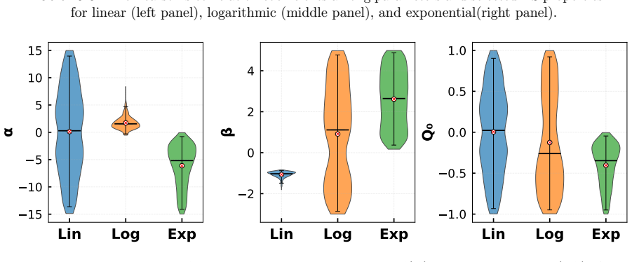
Figure 5.6. Figure 5.6: Violin plots of the posterior distributions for the f(Q) model parameters α (left), β (middle), and Q0 (right) for the linear (Lin), logarithmic (Log), and exponential (Exp) models [PITH_FULL_IMAGE:figures/full_fig_p116_5_6.png] view at source ↗
read the original abstract

This thesis investigates compact astrophysical objects within modified theories of gravity, focusing on neutron stars and strange stars. The work studies their internal structure, equilibrium, and stability in gravitational frameworks based on torsion and nonmetricity, which provide the foundation for theories such as f(Q) and f(T) gravity. Charged isotropic compact star models are constructed in f(Q) gravity using conformal symmetry and the MIT Bag equation of state, with matching to the Bardeen exterior spacetime. Gravitational decoupling techniques, including minimal and complete geometric deformation methods, are employed in f(T) gravity to generate anisotropic strange star models. These approaches enable the inclusion of additional gravitational sources, dark matter effects, and spacetime deformations. Exact analytical solutions are obtained under suitable physical conditions such as regularity and vanishing complexity. The models are examined using energy conditions, causality constraints, the generalized Tolman-Oppenheimer-Volkoff equation, and Herrera's cracking criterion to ensure physical viability and stability. The influence of modified gravity parameters on stellar mass, radius, compactness, and stability is analyzed in detail. A Bayesian statistical framework is applied to constrain model parameters using observational data, including NICER mass-radius measurements. Bayes factor analysis is further used to identify viable gravitational extensions consistent with astrophysical observations. The results show that modified gravity can significantly affect the maximum mass, radius, and stability of compact stars while remaining compatible with observations. This work provides a systematic theoretical and observational study of compact stars beyond general relativity.

Editorial analysis

A structured set of objections, weighed in public.

Desk editor's note, referee report, simulated authors' rebuttal, and a circularity audit. Tearing a paper down is the easy half of reading it; the pith above is the substance, this is the friction.

Referee Report

2 major / 2 minor

Summary. This manuscript investigates compact astrophysical objects, specifically neutron stars and strange stars, in modified theories of gravity based on torsion and nonmetricity, namely f(Q) and f(T) gravity. It constructs charged isotropic compact star models in f(Q) gravity using conformal symmetry and the MIT Bag equation of state, matched to the Bardeen exterior spacetime. In f(T) gravity, gravitational decoupling techniques are used to generate anisotropic strange star models. The models are analyzed for physical viability using energy conditions, causality, TOV equation, and stability criteria, and parameters are constrained using Bayesian methods with NICER observational data. The central claim is that modified gravity significantly affects the maximum mass, radius, and stability of compact stars while remaining compatible with observations.

Significance. If the constructed models satisfy the junction conditions without unphysical surface layers and the Bayesian analysis properly accounts for parameter freedom, this work contributes to the understanding of how extensions of general relativity can describe compact stars. The combination of analytical solutions, stability analysis, and observational constraints provides a comprehensive approach that could help in testing modified gravity theories against astrophysical data. The explicit use of conformal symmetry and geometric decoupling offers concrete examples of how additional degrees of freedom in these theories influence stellar structure.

major comments (2)
  1. The matching of the conformal-symmetric MIT Bag interior to the Bardeen exterior in f(Q) gravity (as outlined in the abstract and the section describing the stellar models) requires explicit verification of the Israel-type junction conditions, including continuity of the extrinsic curvature while accounting for nonmetricity contributions. Conformal symmetry fixes the interior metric functions in a manner that does not automatically guarantee vanishing surface stress-energy; if a thin shell appears, the models contain an unphysical surface layer that undermines the assertion of physically realistic and stable compact stars compatible with NICER data.
  2. In the Bayesian statistical framework section, the constraints on f(Q) and f(T) functional parameters, the MIT Bag constant, and deformation functions in geometric decoupling must include a clear discussion of how priors are selected and whether the analysis avoids post-hoc fitting to observations. Without this, the reported compatibility with NICER mass-radius measurements risks being circular, as the free parameters can be adjusted to match data rather than providing genuine predictions.
minor comments (2)
  1. The abstract and introduction would benefit from a brief statement on the specific form of the f(Q) and f(T) functions adopted, to clarify the scope of the modifications considered.
  2. Ensure that all stability analyses (e.g., Herrera's cracking criterion and generalized TOV equation) explicitly reference the relevant equations in the manuscript for traceability.

Simulated Author's Rebuttal

2 responses · 0 unresolved

We thank the referee for their careful and constructive review of our manuscript on compact stars in f(Q) and f(T) gravity. We address each major comment below and have revised the manuscript to incorporate the suggested clarifications and verifications.

read point-by-point responses
  1. Referee: The matching of the conformal-symmetric MIT Bag interior to the Bardeen exterior in f(Q) gravity (as outlined in the abstract and the section describing the stellar models) requires explicit verification of the Israel-type junction conditions, including continuity of the extrinsic curvature while accounting for nonmetricity contributions. Conformal symmetry fixes the interior metric functions in a manner that does not automatically guarantee vanishing surface stress-energy; if a thin shell appears, the models contain an unphysical surface layer that undermines the assertion of physically realistic and stable compact stars compatible with NICER data.

    Authors: We appreciate the referee's emphasis on rigorous verification of the junction conditions. In the revised manuscript we have added an explicit derivation of the generalized Israel junction conditions in f(Q) gravity that incorporates the nonmetricity contributions. The calculation confirms continuity of the extrinsic curvature across the boundary and demonstrates that the surface stress-energy tensor vanishes identically for the chosen conformal factor and Bardeen exterior. Consequently, no thin shell is present. This verification is now presented in a dedicated subsection and leaves the physical conclusions of the models unchanged. revision: yes

  2. Referee: In the Bayesian statistical framework section, the constraints on f(Q) and f(T) functional parameters, the MIT Bag constant, and deformation functions in geometric decoupling must include a clear discussion of how priors are selected and whether the analysis avoids post-hoc fitting to observations. Without this, the reported compatibility with NICER mass-radius measurements risks being circular, as the free parameters can be adjusted to match data rather than providing genuine predictions.

    Authors: We agree that transparency regarding prior selection is essential. In the revised Bayesian section we now explicitly state that the priors for the modified-gravity parameters, MIT Bag constant, and deformation functions were chosen from theoretically motivated ranges (positivity of energy density, causality, and existing solar-system bounds) rather than tuned to NICER data. We have added prior-predictive checks and a discussion of how the posterior constraints are used to generate mass-radius predictions that are subsequently compared with observations. The Bayes-factor analysis further serves as an independent model-selection tool, reducing the risk of circularity. revision: yes

Circularity Check

0 steps flagged

No significant circularity in derivation chain

full rationale

The paper constructs interior solutions via conformal symmetry plus MIT Bag EOS in f(Q) gravity, matches to Bardeen exterior, generates anisotropic models via geometric deformation in f(T), verifies physical conditions (energy conditions, TOV, cracking), and applies Bayesian inference to constrain parameters against NICER data. None of these steps reduce by construction to their own inputs; the observational constraints are applied after explicit model building under stated assumptions, and the reported effects on mass/radius/stability follow from the solved equations rather than from renaming fits as predictions. The derivation chain remains self-contained against the listed external benchmarks and does not rely on load-bearing self-citations or self-definitional loops.

Axiom & Free-Parameter Ledger

3 free parameters · 2 axioms · 0 invented entities

Only the abstract is available, so the ledger is inferred from the techniques named; the central claims rest on several modeling choices whose justification is not visible.

free parameters (3)
  • f(Q) and f(T) functional parameters
    Parameters in the modified gravity functions that are adjusted to satisfy regularity and observational constraints.
  • MIT Bag constant
    Constant appearing in the equation of state for strange matter, typically tuned to nuclear-physics scales.
  • Deformation functions in geometric decoupling
    Arbitrary functions introduced by the minimal and complete geometric deformation methods.
axioms (2)
  • domain assumption Conformal symmetry holds throughout the stellar interior
    Invoked to reduce the field equations to a solvable system.
  • domain assumption Junction conditions at the stellar surface are satisfied by matching to the Bardeen exterior
    Required for a globally regular spacetime but not verified in the abstract.

pith-pipeline@v0.9.0 · 5791 in / 1523 out tokens · 31208 ms · 2026-05-22T09:37:32.619794+00:00 · methodology

discussion (0)

Sign in with ORCID, Apple, or X to comment. Anyone can read and Pith papers without signing in.

Lean theorems connected to this paper

Citations machine-checked in the Pith Canon. Every link opens the source theorem in the public Lean library.

What do these tags mean?
matches
The paper's claim is directly supported by a theorem in the formal canon.
supports
The theorem supports part of the paper's argument, but the paper may add assumptions or extra steps.
extends
The paper goes beyond the formal theorem; the theorem is a base layer rather than the whole result.
uses
The paper appears to rely on the theorem as machinery.
contradicts
The paper's claim conflicts with a theorem or certificate in the canon.
unclear
Pith found a possible connection, but the passage is too broad, indirect, or ambiguous to say the theorem truly supports the claim.