REVIEW 5 minor 38 references
Regression-adjusted average treatment effect estimates in stratified randomized experiments
T0 review · 0 major / 5 minor · reviewed 2026-08-14 · deepseek-v4-flash
Pith's one-line read In stratified randomized experiments, regression-adjusted estimates of the average treatment effect are consistent, asymptotically normal, and asymptotically no more variable than unadjusted estimates.
desk verdict Solid many-small-strata extension of design-based regression adjustment, but the variance-reduction guarantee requires common treatment proportions and the abstract oversells it. read the letter →
The pith
A machine-rendered reading of the paper's core claim, the machinery that carries it, and where it could break.
The reading
What carries the argument
The load-bearing mechanism is a finite-population central limit theorem for stratified random samples whose main condition is that the largest squared deviation of an outcome from its stratum mean, scaled by $N$, goes to zero; this replaces the usual triangular-array condition with a more interpretable bound. On top of it, the paper studies a weighted linear regression of the outcome on treatment, stratum indicators, centered covariates, and treatment-by-covariate interactions. The variance comparison is carried by the population projections $y_{ij}(z)=y_{i\cdot}(z)+(X_{ij}-X_{i\cdot})^{\top}\beta_z+\varepsilon_{ij}(z)$ for $z=0,1$; because the projection errors are orthogonal to the covariates, the cross terms in $N(\sigma^2_{\mathrm{unadj}}-\sigma^2_{\mathrm{ols}})$ vanish when treatment proportions converge to a common $p$, leaving the nonnegative quadratic form $\sum_i c_i \bar{\beta}_i^{\top}S_{iXX}\bar{\beta}_i/\{p_i(1-p_i)\}$ as the efficiency gain.
What would settle it
Consider a two-stratum design with $p_1\to 0.2$, $p_2\to 0.8$, a strong covariate in both strata, and bounded potential outcomes, and compute the limit of $N(\sigma^2_{\mathrm{ols}}-\sigma^2_{\mathrm{unadj}})$ from the paper's formulas; if any such sequence makes that limit positive, the 'never worse' claim fails. A simulation under Conditions 1--6 should also show $\hat{\sigma}^2_{\mathrm{ols}}\le \hat{\sigma}^2_{\mathrm{unadj}}$ in probability; a configuration where the adjusted interval is systematically wider would delimit the theorem.
Extended reading notes
Core claim
The paper's central claim is that covariate adjustment after stratified randomization is asymptotically no worse than stratification alone. Its main result, Theorem 3, states that under Conditions 1--6, with at least two treated and two control units per stratum, $(\hat{\tau}_{\mathrm{ols}}-\tau)/\sigma_{\mathrm{ols}}$ converges in distribution to $N(0,1)$, and if $p_i$ converges uniformly to a common $p$, the difference between the asymptotic variances of $\sqrt{N}\hat{\tau}_{\mathrm{ols}}$ and $\sqrt{N}\hat{\tau}_{\mathrm{unadj}}$ is the limit of $-\sum_i c_i \bar{\beta}_i^{\top}S_{iXX}\bar{\beta}_i/\{p_i(1-p_i)\}\le 0$, where $\bar{\beta}_i=(1-p_i)\beta_1+p_i\beta_0$ combines the population projection coefficients for treatment and control. Theorem 2 supplies the supporting finite-population central limit theorem for the unadjusted estimator, allowing the number of strata to tend to infinity. The paper also proves an analogous result, Theorem 4, for a stratum-interacted estimator in designs with a few large strata, and provides conservative variance estimators that yield large-sample confidence intervals with at least nominal coverage.
Load-bearing premise
The headline guarantee that regression adjustment never increases variance depends on every stratum's treatment fraction converging to the same number $p$; if treatment fractions stay different across strata, extra terms appear in the variance comparison that the proof does not control.
Editorial extensions
If this is right
- In experiments with many small strata, researchers can use $\hat{\tau}_{\mathrm{ols}}$ with the conservative variance estimator $\hat{\sigma}^2_{\mathrm{ols}}$; the resulting intervals have asymptotic coverage at least nominal and are asymptotically no wider than intervals from $\hat{\tau}_{\mathrm{unadj}}$.
- Even when treatment proportions differ across strata, the stratified difference-in-means estimator is consistent and asymptotically normal, so the paper's central limit theorem applies to designs with many small strata; only the variance-reduction claim needs the common-$p$ condition.
- With a few large strata and heterogeneous covariate-outcome relationships, the stratum-interacted estimator $\hat{\tau}_{\mathrm{ols,int}}$ is asymptotically at least as efficient as the common-coefficient estimator $\hat{\tau}_{\mathrm{ols}}$.
- The conservative variance estimators mean confidence intervals based on the adjusted estimators are asymptotically at least as short as those based on the unadjusted estimator, in line with the simulations showing 4--19% shorter intervals.
Reading between the lines
- Beyond the paper's equal-$p$ condition, a direct numerical study of the cross terms in $N(\sigma^2_{\mathrm{ols}}-\sigma^2_{\mathrm{unadj}})$ could show whether the no-worse guarantee survives when treatment shares differ across strata; the paper's proof does not cover that case.
- The variance-difference formula identifies exactly where efficiency gains come from, so before fitting the adjusted regression one could compute a sample analogue of $\sum_i c_i \bar{\beta}_i^{\top}S_{iXX}\bar{\beta}_i/\{p_i(1-p_i)\}$ as a planning diagnostic for how much a given covariate is worth.
- An immediate extension the paper leaves open is high-dimensional regression adjustment; its projection-and-residual argument would need a concentration inequality for stratified sampling, and the paper names that as the main technical obstacle.
Signed reviews
Editorial analysis
A structured set of objections, weighed in public.
Referee Report
Summary. The paper develops randomization-based inference for average treatment effects in stratified randomized experiments, allowing the number of strata to grow with the sample size. It re-establishes a finite-population central limit theorem for stratified samples (Theorem 1), proves asymptotic normality and conservative variance estimation for the stratified difference-in-means estimator (Theorem 2), and analyzes regression adjustment with treatment-by-covariate interactions (Theorem 3). Under Conditions 1–6, the regression-adjusted estimator is consistent and asymptotically normal; when the stratum-specific treatment proportions converge uniformly to a common limit, its asymptotic variance is no larger than that of the unadjusted estimator, and a conservative variance estimator is provided. A second estimator with stratum-specific regression coefficients is treated for the few-large-strata regime (Theorem 4 and Corollary 1). Simulations and an application to an iron-deficiency schooling trial illustrate the methods.
Significance. If the results hold, this is a valuable extension of the completely randomized regression-adjustment theory of Lin and of Li and Ding to stratified designs with many small strata. The paper gives precise conditions, a transparent variance decomposition, and conservative variance estimators that support large-sample confidence intervals, and it carefully distinguishes the regimes where common regression coefficients versus stratum-specific coefficients are appropriate. The proof appendix is detailed and largely self-contained, and the simulation study covers several design regimes with results that match the theoretical predictions. The main caveat—that the advertised variance reduction for the first estimator requires the asymptotic treatment proportions to be common across strata—is explicitly stated in Condition 1 and Remark 3, although it is underemphasized in the abstract and in the empirical discussion.
minor comments (5)
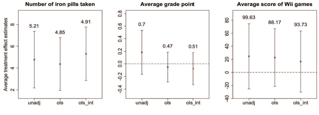
- [Abstract and Section 6] The abstract states that the asymptotic variance of the regression-adjusted estimator is 'no greater' than that of the difference-in-means estimator without mentioning the condition pi,infinity = p. This is a genuine scope restriction: Theorem 3 establishes the variance-reduction claim only under this condition, and the application in Section 6 uses strata with pi ranging from 0.636 to 0.688, so the reported shorter confidence intervals for tau_ols are not formally covered by the theorem. Please qualify the abstract and add a sentence in Section 6 noting that the efficiency gain there is empirical rather than guaranteed by Theorem 3.
- [Remark 3] Remark 3 correctly acknowledges that the efficiency improvement requires pi to tend uniformly to a common limit, but the discussion would be strengthened by stating explicitly that, when treatment proportions differ across strata, the cross terms 2*sum_i c_i p_i^{-1} S_iXepsilon(1)^T beta_i and 2*sum_i c_i (1-p_i)^{-1} S_iXepsilon(0)^T beta_i need not vanish and are not sign-definite, so no no-worse claim is made in that case.
- [Section 4.2, equation for tau_i,ols_int] In the definition of tau_i,ols_int, the second term appears to contain a typo: it reads {yhat_i.(0) - X_i.}^T betahat_0i, which should presumably be {Xhat_i.(0) - X_i.}^T betahat_0i, matching the treatment-group expression and the preceding text.
- [Appendix, Proof of Theorem 3] There is a minor typo: 'Thereom 2' should be 'Theorem 2'. Also, in the proof of Lemma 1, the bound in equation (18) is clear, but the sentence following it could state explicitly which quantities are bounded by Condition 1 and Condition 9, since the current wording is slightly compressed.
- [Theorem 1] The condition for the consistency of the variance estimator is stated as 2 <= n1i <= ni - 2 for every stratum, which requires at least two treated and two control units. This is noted in Remark 2, but it would be helpful to repeat the restriction in Theorem 1's statement so that the reader immediately sees the difference from the Bickel-Freedman result cited.
Circularity Check
No significant circularity: the central theorems are proved from independent external benchmarks and from algebraic properties of population projections, not by fitting the conclusions into the inputs.
full rationale
The load-bearing results are self-contained arguments built on external benchmarks. Theorem 1 is proved by showing that the paper's condition m1N/N -> 0 implies the Lindeberg-Feller condition of Bickel and Freedman [4], an independent finite-population central limit theorem; the paper explicitly says 'Our proof relies on the following finite population central limit theorem proved by Bickel and Freedman [4]'. Theorem 2 applies Theorem 1 to the constructed population Pi_a, with Conditions 1-3 ensuring that the needed moment and distance conditions hold; this is a direct derivation, not a circular one. Theorem 3 defines tau_ols as the ordinary least squares estimator from a weighted regression with treatment-by-covariate interactions, and the population projection coefficients beta_1, beta_0 are fixed minimizers of deterministic weighted least squares criteria. The variance comparison is obtained by decomposing N*sigma2_unadj - N*sigma2_ols into a nonnegative quadratic term plus cross terms that vanish because sum_i c_i S_iXepsilon(1) = 0 and because Condition 1 with p_i,infty = p gives uniform convergence beta_i/p_i - beta_infty/p -> 0. That the cross terms vanish in this way is shown by the paper's own algebra, not by defining sigma2_ols to match sigma2_unadj. The consistency of the variance estimators is proved from Lemmas 1 and 2, which are established from sampling theory, and from the Bickel-Freedman CLT, rather than from the conclusion being estimated. Theorem 4 explicitly relies on Proposition 3 of Li and Ding [20], an independent published result, and is a straightforward extension to independent large strata. The only self-citation, reference [22], appears in the Discussion as a pointer to high-dimensional extensions and is not load-bearing for any theorem. The stated restriction that the no-worse-variance claim requires asymptotically common treatment proportions p_i,infty = p is a genuine scope condition, explicitly acknowledged in Condition 1, Theorem 3, and Remark 3; it limits the applicability of the efficiency claim but does not make the derivation circular. No fitted parameter is renamed as a prediction, and no claimed result reduces by construction to its own inputs.
Assumptions & free parameters
assumptions (6)
- domain assumption Potential outcomes and covariates are fixed finite-population quantities; randomness arises only from treatment assignment (Neyman-Rubin model).
- domain assumption Stable unit treatment value assumption (SUTVA), with no interference and no hidden treatment versions.
- domain assumption Condition 1: treatment proportions pi are bounded away from 0 and 1 and converge to limits; for Theorem 3, they converge to a common p.
- domain assumption Condition 2: maximum within-stratum squared deviations of potential outcomes are o(N).
- domain assumption Conditions 4-6: covariates have vanishing maximum squared deviation relative to N, and the weighted covariance matrix converges to a finite invertible limit.
- standard math Bickel and Freedman's finite-population central limit theorem is accepted as an external theorem.
Cite this review
Pith. "Pith review of Regression-adjusted average treatment effect estimates in stratified randomized experiments." pith.science (2026). https://pith.science/paper/FOUFZOTR
@misc{pith2026190801628,
  author       = {Pith},
  title        = {Pith review of: Regression-adjusted average treatment effect estimates in stratified randomized experiments},
  year         = {2026},
  howpublished = {\url{https://pith.science/paper/FOUFZOTR}},
  note         = {Machine review of arXiv:1908.01628}
}
read the original abstract
Researchers often use linear regression to analyse randomized experiments to improve treatment effect estimation by adjusting for imbalances of covariates in the treatment and control groups. Our work offers a randomization-based inference framework for regression adjustment in stratified randomized experiments. Under mild conditions, we re-establish the finite population central limit theorem for a stratified experiment. We prove that both the stratified difference-in-means and the regression-adjusted average treatment effect estimators are consistent and asymptotically normal. The asymptotic variance of the latter is no greater and is typically lesser than that of the former. We also provide conservative variance estimators to construct large-sample confidence intervals for the average treatment effect.
Figures


Reference graph
Works this paper leans on
-
[1]
Abadie, A. and Imbens, G. W. (2008). Estimation of the con ditional variance in paired experiments. Ann. Econ. Statist., 91/92:175–87
work page 2008
-
[2]
Angrist, J. D. and Imbens, G. W. (1995). Two-stage least s quares estimation of average causal effects in models with variable treatment intensity. Journal of the American Statistical Association , 90(430):431–442
work page 1995
-
[3]
Angrist, J. D., Imbens, G. W., and Rubin, D. B. (1996). Ide ntification of causal effects using instrumental variables. Journal of the American Statistical Association , 91(434):444–455
work page 1996
-
[4]
Bickel, P . J. and Freedman, D. A. (1984). Asymptotic norm ality and the bootstrap in stratified sampling. Ann. Statist., 12:470–82
work page 1984
-
[5]
Bloniarz, A., Liu, H., Zhang, C. H., Sekhon, J., and Y u, B. (2016). Lasso adjustments of treatment effect estimates in randomized experiments. Proc. Natl. Acad. Sci. U.S.A. , 113:7383–90. 18
work page 2016
-
[6]
Chong, A., Cohen, I., Field, E., Nakasone, E., and Torero , M. (2016). Iron deficiency and schooling attainment in peru. Am. Econ. J. Appl. Econ , 8:222–55
work page 2016
-
[7]
Cochran, W. G. (1977). Sampling Techniques. New Y ork: Wiley, 3rd edition
work page 1977
-
[8]
Fisher, R. A. (1926). The arrangement of field experiment s. J. Min. Agric. Gt Br ., 33:503–13
work page 1926
Show all 38 references
-
[9]
Fogarty, C. B. (2018a). On mitigating the analytical lim itations of finely stratified experiments. J. R. Statist. Soc. B, 80:1035–56
2018
-
[10]
Fogarty, C. B. (2018b). Regression-assisted inferenc e for the average treatment effect in paired experiments. Biometrika, 105:994–1000
2018
-
[11]
Freedman, D. A. (2008a). On regression adjustments in e xperiments with several treatments. The Annals of Applied Statistics, 2:176–196
2008
-
[12]
Freedman, D. A. (2008b). Randomization does not justif y logistic regression. Statistical Science, 23:237–249
2008
-
[13]
Gerber, A. S. and Green, D. P . (2012). Field Experiments: Design, Analysis and Interpretation . New Y ork: Norton
2012
-
[14]
J., S¨ avje, F., and Sekhon, J
Higgins, M. J., S¨ avje, F., and Sekhon, J. S. (2015). Blo cking estimators and inference under the neyman–rubin model. arXiv: 1510.01103
2015 arXiv
-
[15]
Imai, K. (2008). V ariance identification and efficiency analysis in randomized experiments under the matched- pair design. Statist. Med., 27:4857–73
2008
-
[16]
Imai, K., King, G., and Stuart, E. A. (2008). Misunderst andings between experimentalists and observationalists about causal inference. J. R. Statist. Soc. A , 171:481–502
2008
-
[17]
Imbens, G. W. and Angrist, J. D. (1994). Identification a nd estimation of local average treatment effects. Econometrica, 62(2):467–475
1994
-
[18]
Imbens, G. W. and Rubin, D. B. (2015). Causal Inference for Statistics, Social, and Biomedical Sc iences: An Introduction. New Y ork: Cambridge University Press
2015
-
[19]
Kempthorne, O. (1955). The randomization theory of exp erimental inference. J. Am. Statist. Assoc., 50:946–67
1955
-
[20]
and Ding, P
Li, X. and Ding, P . (2017). General forms of finite popula tion central limit theorems with applications to causal inference. J. Am. Statist. Assoc. , 112:1759–69
2017
-
[21]
Lin, W. (2013). Agnostic notes on regression adjustmen ts to experimental data: Reexamining Freedman’s critique. Ann. Appl. Statist., 7:295–318
2013
-
[22]
and Y ang, Y
Liu, H. and Y ang, Y . (2018). Penalized regression adjusted causal effect estimates in high dimensional random- ized experiments. arXiv preprint arXiv:1809.08732
2018 arXiv
-
[23]
W., Sekhon, J
Miratrix, L. W., Sekhon, J. S., and Y u, B. (2013). Adjust ing treatment effect estimates by post-stratification in randomized experiments. J. R. Statist. Soc. B , 75:369–96. 19
2013
-
[24]
Moore, K. L. and van der Lann, M. J. (2009). Covariate adj ustment in randomized trials with binary outcomes: targeted maximum likelihood estimation. Statistics in Medicine, 28:39–64
2009
-
[25]
Morgan, K. L. and Rubin, D. B. (2012). Rerandomization t o improve covariate balance in experiments. Ann. Statist., 40:1263–82
2012
-
[26]
Neyman, J. (1935). Statistical problems in agricultur al experimentation (with discussion). Supplement to J. R. Statist. Soc., 2:107–80
1935
-
[27]
M., and Speed, T
Neyman, J., Dabrowska, D. M., and Speed, T. (1990). On th e application of probability theory to agricultural experiments. Statist. Sci., 5:465–72
1990
-
[28]
Pashley, N. E. and Miratrix, L. W. (2017). Insights on va riance estimation for blocked and matched pairs designs. arXiv: 1710.10342
2017 arXiv
-
[29]
Robinson, J. (1978). An asymptotic expansion for sampl es from a finite population. Ann. Statist., 6:1005–11
1978
-
[30]
Rubin, D. B. (1974). Estimating causal effects of treat ments in randomized and nonrandomized studies. J. Educ. Psychol., 66:688–701
1974
-
[31]
Rubin, D. B. (1980). Randomization analysis of experim ental data: the fisher randomization test comment. J. Am. Statist. Assoc., 75:591–93
1980
-
[32]
Schochet, P . Z. (2016). Statistical theory for the rct- yes software: Design-based causal inference for the rcts, second edition. Technical report, Washington, DC: U.S. Department of Education, Institute of Education Sciences, National Center for Education Evaluation and Regi...
2016
-
[33]
Sen, P . K. (1995). The H´ ajek asymptotics for finite popu lation sampling and their ramifications. Kybernetika, 31:251–68
1995
-
[34]
Y ue, L., Li, G., Lian, H., and Wan, X. (2019). Regression adjustment for treatment effect with multicollinearity in high dimensions. Computational Statistics & Data Analysis , 134:17–35
2019
-
[35]
A., and Davidian, M
Zhand, M., Tsiatis, A. A., and Davidian, M. (2008). Impr oving efficiency of inferences in randomized clinical trials using auxiliary covariates. Biometrics, 55:707–715
2008
-
[36]
variance weight
Zhao, A., Ding, P ., Mukerjee, R., and Dasgupta, T. (2018 ). Randomization-based causal inference from split- plot designs. Ann. Statist., 46(5):1876–903. A. Proof of main theorems Proof of Theorem 1 Proof 1 Our proof relies on the following finite population central l imit the...
2018
-
[37]
holds, which further implies that the Lindeberg–Feller condition holds. Proof of Theorem 2 Proof 2 We write ˆτi· − τi· as the average of a stratified random sample: ˆτi· − τi· = ni∑ j=1 { Zijyij(1) n1i − (1 − Zij)yij(0) n0i } − {yi·(1) − yi·(0)} = ni∑ j=1 [ Zij{yij(1) − yi·(1)}...
-
[38]
Proof of lemmas Proof of lemma 1 Proof 6 Applying standard sampling theory (see for example Cochran [7]), it is easy to show that the mean of sibd is Sibd, i.e., E(sibd) = Sibd
and (14), we have B∑ i=1 ci { S2 iε(1)/p + S2 iε(0)/(1 − p) } − B∑ i=1 ci { S2 iη(1)/p + S2 iη(0)/(1 − p) } = 1 p B∑ i=1 ci ( β1i − β1 ) T SiXX ( β1i − β1 ) + 1 1 − p B∑ i=1 ci ( β0i − β0 ) T SiXX ( β0i − β0 ) ≥ 0, since the covariance matrix SiXX is positive-definite. Proof of...
Reviewed August 14, 2026 · model on record in the stance chip above.
Discussion (0). Continue with ORCID to comment.