Estimation of the Number of Components of Non-Parametric Multivariate Finite Mixture Models

Caleb Kwon; Eric Mbakop

REVIEW 3 major objections 5 minor 45 references

Estimation of the Number of Components of Non-Parametric Multivariate Finite Mixture Models

T0 review · 3 major / 5 minor · reviewed 2026-08-14 · deepseek-v4-flash

Challenge this review Re-run · record.json Download PDF Read on arXiv ↗ Review JSON

Pith's one-line read The number of mixture components equals the rank of an integral operator, and singular-value thresholding estimates it consistently.

desk verdict A solid operator-rank method for estimating the number of mixture components, with a real gap between the threshold that is proved and the one that is implemented; deserves refereeing but needs the claims realigned with the guarantees. read the letter →

arxiv 1908.03656 v2 pith:FSHTHEW7 submitted 2019-08-10 stat.ME math.STstat.TH

Caleb Kwon , Eric Mbakop This is my paper · ORCID

classification stat.MEmath.STstat.TH MSC 62G0562G1562H3047A5547G1047N30

keywords finitemixturemodelnumberofcomponentsnonparametricconditionalindependencemultivariatedataintegraloperatorsingularvaluethresholdinglatentvariable

verification ladder T0 review T1 audit T2 compute T3 formal

The pith

A machine-rendered reading of the paper's core claim, the machinery that carries it, and where it could break.

The reading

This paper claims that in a multivariate finite mixture model with repeated conditionally independent measurements, the unknown number of mixture components $M$ is exactly the rank of an integral operator $T$ built from the joint density of the observed variables. Because $T$ is identified from data and its singular values are stable under small perturbations, the paper estimates $M$ by counting how many singular values of a kernel-smoothed empirical version of $T$ exceed a data-driven threshold. The authors prove consistency of this count and give finite-sample probability bounds, and their simulations show good performance at moderate sample sizes. The method matters because it removes the need to know $M$ in advance or to choose a partition of the support, a common bottleneck in estimating finite mixture models.

What carries the argument

The central object is the integral operator $T$ with kernel equal to the joint density: $[T(u)](x_2)=\int u(x_1)f(x_1,x_2)\,dx_1$. Conditional independence and the mixture representation decompose $T$ into $M$ rank-one tensor products, so its rank counts the number of components. Because estimating $T$ directly introduces a bias whose rate depends on unknown smoothness, the paper uses the regularized operator $T_h$ obtained by convolving the density with a product kernel; $T_h$ has the same rank as $T$ and is unbiasedly estimated by $\widehat T_h$. The argument then runs on two inequalities: the Hoffman-Wielandt inequality, which controls how much tail sums of singular values change under Hilbert-Schmidt perturbations, and concentration inequalities for sums of independent Hilbert-space-valued random variables, which yield the explicit threshold $\widehat\tau_h(N,\delta)$. Computationally, the singular values of $\widehat T_h$ equal those of an $N\times N$ matrix built from kernel evaluations, so the whole procedure reduces to standard matrix computations.

What would settle it

Run the estimator on the paper's Design 2, a mixture of three uniform components with disjoint supports and equal weights $1/3$. There the nonzero singular values of $T$ are exactly $1/3$ by the closed-form calculation in Remark 2.2, so the theory predicts $\widehat M=3$ with probability approaching 1; the paper reports 100% at $N=2000$. If a faithful replication instead systematically selected fewer than three components, the spectral thresholding logic would be wrong, and any design satisfying Assumption 2.1 with a provably positive smallest nonzero singular value but where the estimator converges to a smaller number would expose a gap in the non-asymptotic bound.

Watch

Extended reading notes

Core claim

Under Assumption 2.1, that the conditional distributions of at least two observed components are linearly independent across the $M$ latent groups, the integral operator defined by $[T(u)](x_2)=\int u(x_1)f(x_1,x_2)\,dx_1$ has finite rank exactly $M$. The mixture representation makes $T$ a sum of $M$ rank-one operators $\pi_m f_m^2\otimes f_m^1$, and linear independence prevents the rank from collapsing. The estimator works with a kernel-smoothed version $T_h$, which has the same rank as $T$ and admits an unbiased empirical counterpart $\widehat T_h$ from an i.i.d. sample. The estimator is $\widehat M=\#\{j: (\sum_{i\ge j}\sigma_i(\widehat T_h)^2)^{1/2}\ge \widehat\tau_h(N,\delta)\}$, where $\widehat\tau_h$ is a data-driven upper bound on the Hilbert-Schmidt estimation error. Theorem 3.1 shows $P(\widehat M=\mathrm{rank}(T))\to 1$ when $\delta(N)\to0$ and $\ln(1/\delta(N))=o(N)$, so $\widehat M$ consistently estimates $M$ under Assumption 2.1.

Load-bearing premise

The load-bearing premise is that across the latent groups, the conditional distributions of at least two observed variables are genuinely distinct (no group's distribution is a mixture of the others'), because if that fails the operator's rank falls below $M$ and the estimator can only claim a lower bound.

Editorial extensions

If this is right

The number of mixture components is identifiable from the joint distribution alone whenever two conditional distributions are linearly independent, with no parametric model for the component densities and no need to preselect a partition or an upper bound $M_0$.
The estimator is consistent at essentially parametric concentration rates: $P(\widehat M=M)\to1$ as long as $\delta(N)\to0$ and $\ln(1/\delta(N))=o(N)$, and the finite-sample bound shows how large $N$ must be relative to the smallest nonzero singular value.
Overestimation is controlled by design: with probability at least $1-2\delta$, $\widehat M$ is no larger than the true rank, so the method is conservative when the smallest nonzero singular value is close to the estimation-error threshold.
When the linear-independence assumption fails, $\widehat M$ still consistently estimates a lower bound on $M$, and this lower bound is at least as large as the one from partition-based rank estimation.
For $K>2$, the same construction applied to all pairs of variables, or to two groups of variables, and taking the maximum estimated rank yields a consistent estimator of $M$ under the appropriate independence assumption.

Reading between the lines

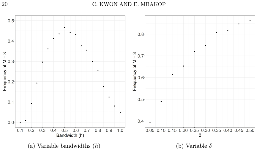
Editorial extensions of the paper, not claims the author makes directly.

The threshold in Theorem 3.1 is a worst-case concentration bound, and the simulations show it is loose; a practical extension is to choose the threshold from the estimated singular-value spacings or to calibrate $\delta$ upward when underestimation is the main risk.
The same rank-of-a-sum-of-rank-one-operators view could carry over to other order-selection problems, such as factor models, hidden Markov models, or tensor decompositions, where the object of interest is a low-rank operator assembled from conditionally independent measurements.
A natural diagnostic suggested by the proofs is to report the estimated smallest nonzero singular value alongside $\widehat M$, since the separation between that value and the threshold determines whether the estimate is an exact count or merely a lower bound.
Bandwidth choice remains open in the paper; an automatic rule that selects $h$ to maximize the gap between estimated singular values is a testable next step.

Share X Bluesky LinkedIn Reddit HN

Signed reviews

No signed human review yet.

Editorial analysis

A structured set of objections, weighed in public.

Desk editor's note, referee report, and a circularity audit.

Desk Editor's Note

read the letter

Bottom line: this is a genuine contribution with an honest gap between what is proved and what is implemented. The identification result is clean: under linear independence, the number of components M equals the rank of an integral operator T built from the pairwise density, and the proofs in Section 2 are careful. The genuinely new content is the estimator, which counts tail sums of singular values of a kernel-smoothed empirical operator above a data-driven threshold, with non-asymptotic concentration bounds. That is a real step beyond Kasahara-Shimotsu, whose rank-based estimator is only a lower bound unless the analyst happens to choose a good partition, and whose results are asymptotic only. Proposition 2.1 is explicitly an alternative proof of a known identification fact; the contribution is the estimator and its finite-sample guarantees, and that is where the paper earns its keep. The simulations are honest, including Design 1, where the method selects the true M only 40% of the time at N=2000; the paper attributes this to the tiny third singular value rather than hiding it. I found no circularity: rank(T)=M is derived from the mixture representation, not assumed, and the threshold is data-driven through concentration inequalities rather than fit to match the answer. The citation pattern is appropriate, and the self-citation to Mbakop's thesis is used where needed.

The soft spot is the one the stress-test flags, and it is real. Theorem 3.1 proves consistency for the explicit threshold in equation (3.8), with h treated as fixed. The implementation and the recommended procedure use equation (3.24), which is obtained by replacing sigma_h^2 with its sample analogue and then dropping the term (L_hat_h^2/2) sqrt(ln(1/delta)/N). The paper itself says that drop is "not justified by our results." So the high-probability event that the estimation error is bounded by the threshold, which is the load-bearing step, is not established for the implemented threshold. The same goes for the bandwidth: the theorem fixes h, while the simulations use Silverman's rule, which is data-dependent, and no uniform-in-h or data-dependent-h argument is supplied. This is not an internal contradiction in the theorem, but it means the abstract's claim that "our estimator of M is consistent" applies to a different estimator from the one whose finite-sample performance is reported. I do not doubt that the implemented estimator is consistent; the gap is that the paper has not shown it.

Who this is for: econometricians and statisticians working on nonparametric multivariate mixtures, especially empirical IO and auction settings where the number of latent types matters. It deserves a serious referee, not a desk reject. My recommendation: send it out, but the revision should either prove a bound for the (3.24) threshold or reposition the consistency claim so it covers only the procedure with the proved threshold. Conditional accept, not reject.

Referee Report

3 major / 5 minor

Summary. The paper proposes a nonparametric estimator for the number of components M in a finite mixture model where K ≥ 2 observed variables are conditionally independent given a finitely supported latent variable. Under a linear-independence assumption on two component distribution families (Assumption 2.1), the paper proves that an integral operator T identified from the joint density has rank exactly M. The estimator regularizes T through a kernel convolution to obtain operators T_h, estimates them from an i.i.d. sample via $\hat T_h$, and estimates M by counting how many tail sums of squared singular values of $\hat T_h$ exceed a data-driven threshold. The main theoretical result, Theorem 3.1, gives non-asymptotic probability bounds and establishes consistency of $\hat M$ when the threshold is defined by Eq. (3.8), h is fixed, and $\delta=\delta(N)\to 0$ with $\ln(1/\delta)=o(N)$. The paper also provides an efficient matrix implementation of the singular value computation (Corollary 3.1) and reports Monte Carlo and empirical results using a different threshold rule (Eq. 3.24) and a data-dependent bandwidth selected by Silverman's rule.

Significance. If the consistency result can be extended to the actual implemented procedure, this would be a valuable contribution to the literature on estimating the number of mixture components. The rank-identification argument is elegant and avoids the need to choose a partition, unlike the method of Kasahara and Shimotsu (2014), which in general only estimates a lower bound unless a favorable partition is known. The paper also provides finite-sample guarantees through concentration inequalities, a computational procedure for the singular values, and extensive simulations covering several designs. The strengths include the clear use of operator perturbation theory and the explicit, machine-checkable derivations of the rank preservation (Propositions 2.1--2.6) and the matrix representation in Corollary 3.1.

major comments (3)

[Section 3.2, Eq. (3.24)] The implemented and recommended threshold is not justified by the theory. Theorem 3.1 establishes consistency for the threshold $\hat\tau_h(N,\delta)$ defined in Eq. (3.8), but Section 3.2 replaces the population quantity $\sigma_h^2$ by its sample analogue and then explicitly drops the term $(\hat L_h^2/2)\sqrt{\ln(1/\delta)/N}$ from $\hat\Sigma_h^2$. The paper itself states that this change "is not justified by our results." Consequently, the key event $\{\|\hat T_h - T_h\|_{HS} \le \hat\tau(N,\delta)\}$ is not shown to hold for the implemented threshold, so neither the lower-bound inequality (3.11) nor the consistency conclusion transfers to the estimator actually used in the Monte Carlo study and the empirical examples. This gap is load-bearing because the abstract claims "we prove that our estimator of M is consistent" while the paper's own recommendation and all numerical results use the unjustified threshold.
[Theorem 3.1 vs. Section 4 implementation] Theorem 3.1 treats the bandwidth h as fixed, whereas the recommended implementation (Section 4) selects h by Silverman's rule, a data-dependent quantity. Since the threshold $\hat\tau_h(N,\delta)$ and the concentration bounds depend on h through $L_h$ and $\sigma_h^2$, no uniform-in-h or data-dependent-h argument is supplied. As a result, the consistency proof does not cover the bandwidth selection used in the simulations and applications, and the paper itself acknowledges in Remark 3.4 that the question of good data-driven choices of h is left for future research. This further separates the theoretical guarantee from the reported finite-sample performance.
[Abstract and Remark 3.3] The consistency claim in the abstract and introduction is stated without the qualification that the theorem requires $\delta=\delta(N)\to 0$ with $\ln(1/\delta)=o(N)$, and the simulation study and empirical examples use fixed values of $\delta$ (0.05 and 0.4). Remark 3.3 does note the asymptotic condition on $\delta$, but the paper does not explain whether the fixed $\delta$ used in the recommended procedure is meant as a finite-sample tuning parameter or as a sequence that would need to decay to zero for consistency. The current presentation invites the reader to conclude that the implemented procedure with fixed $\delta$ is covered by the theorem, which is not the case. This is a substantive mismatch between the theoretical scope and the practical recommendation.

minor comments (5)

[Section 2.2, Eq. (2.12)] In the definition of the operator $T_{i,j}$, the integration variable in the displayed formula is written as $dx_j$, but it should be $dx_i$ because the operator maps $L^2(S_i)$ to $L^2(S_j)$.
[Section 7, proof of Proposition 3.1] The proof first cites "Theorem 3.4 of Pinelis [28]" and then later refers to "Theorem 3.2 of Pinelis [28]"; this appears to be an inconsistent citation, and the authors should verify which theorem number is intended.
[Section 4 and 5] The name "Kashara and Shimotsu" is repeatedly misspelled (e.g., "Kashara and Shimotsu's" in Sections 4, 5.1, and 5.2); it should be "Kasahara and Shimotsu."
[Section 4, Table 1] The row label "SVT" is used for the proposed method in the simulation tables, but this abbreviation is not defined in the text; it should be introduced (e.g., "singular value thresholding").
[Section 3, Eq. (3.7) and Eq. (3.8)] There are minor typographical errors in the displayed formulas: the expression $2L_h\ln(2/\delta))/N$ contains an extra closing parenthesis, and the square-root expression in Eq. (3.8) is formatted unclearly. These should be cleaned up.

Circularity Check

0 steps flagged · score 1.0 of 10

No circularity: the operator-rank identification and thresholding estimator are derived from the mixture structure and concentration inequalities; the only self-citation is non-load-bearing.

full rationale

The derivation is self-contained. T is defined from the mixture density, equation (2.2) follows from (1.1) by expanding the joint density, and Proposition 2.1 proves rank(T) ≤ M and rank(T) = M under Assumption 2.1 by constructing dual elements ω_m rather than assuming the rank. The estimator (3.10) counts singular-value tail sums of a consistent estimator T̂_h against a data-driven threshold built from a concentration inequality (Proposition 3.1 and equation 3.8). No parameter is fitted to M; δ is chosen by the analyst and controls the overestimation probability through inequality (3.11). The proof of Theorem 3.1 uses the Hoffman-Wielandt inequality together with the bound ||T̂_h − T_h||_HS ≤ τ̂_h(N,δ), and τ̂_h is not constructed from M or from the singular values of T. The one self-citation, Mbakop [25], supports only the assertion that Assumption 2.1 is mild and holds generically; it is not used in the consistency proof and can be removed without changing Theorem 3.1. The paper explicitly flags that the implemented threshold (3.24) drops a term that is 'not justified by our results'; that is a gap between the proved estimator and the recommended implementation, not a circular reduction, because the implemented threshold remains an upper-bound procedure whose value is not chosen to match the target M. No circular step is present.

Assumptions & free parameters 3 free parameters · 6 assumptions · 0 invented entities

The central claim rests on standard singular value perturbation theory and concentration inequalities, plus the domain assumption of linear independence. The only analyst-chosen inputs are kernel, bandwidth, and threshold confidence level; these are tuning parameters rather than fitted parameters, so the identification argument does not hide free parameters. No new entities are postulated.

free parameters (3)

Bandwidth h = Silverman's rule h ~ N^{-1/6} for X in R^2
The estimator and threshold depend on a kernel bandwidth h. Consistency holds for any fixed h, but finite-sample performance and threshold magnitude depend on h. No optimal data-driven h is provided, and the theory is only for fixed h.
Tuning parameter delta = 0.05 and 0.40 in simulations
User-chosen confidence parameter controlling overestimation probability. Consistency requires delta(N) -> 0 with ln(1/delta(N)) = o(N).
Kernel K = Gaussian
Any kernel with Fourier transform vanishing on a null set preserves rank. Gaussian is chosen for closed-form phi_h. Performance may depend on the choice.

assumptions (6)

standard math Hoffman-Wielandt inequality for singular values of finite-rank operators and Weyl's inequality.
Used in Section 2.1 to relate singular value perturbation to operator norm and Hilbert-Schmidt norm error.
standard math Concentration inequalities for sums of independent Hilbert space valued random elements (Pinelis 1994; Smale and Zhou 2007).
Used in Proposition 3.1 to derive data-driven bounds on the estimation error of T-hat_h.
standard math Fourier transform invertibility and convolution properties.
Used in Proposition 2.2 to show rank(T_h) = rank(T) when the kernel Fourier transform vanishes only on a null set.
domain assumption Assumption 2.1: linear independence of the conditional distributions of at least two components.
Needed for rank(T) = M; without it the estimator is consistent only for a lower bound on M.
domain assumption Model (1.1): conditional independence of K observed variables given a finitely supported latent variable.
This is the defining structure of the mixture model under study.
domain assumption The density f is square integrable, and the kernel K lies in L1(R) intersect L2(R) with Fourier transform vanishing on a null set.
Required for T to be Hilbert-Schmidt and for the regularization to preserve rank.

how reviews work

0 comments

Cite this review

Pith. "Pith review of Estimation of the Number of Components of Non-Parametric Multivariate Finite Mixture Models." pith.science (2026). https://pith.science/paper/FSHTHEW7

@misc{pith2026190803656,
  author       = {Pith},
  title        = {Pith review of: Estimation of the Number of Components of Non-Parametric Multivariate Finite Mixture Models},
  year         = {2026},
  howpublished = {\url{https://pith.science/paper/FSHTHEW7}},
  note         = {Machine review of arXiv:1908.03656}
}

abstract

We propose a novel estimator for the number of components (denoted by $M$) in a K-variate non-parametric finite mixture model, where the analyst has repeated observations of $K\geq2$ variables that are independent given a finitely supported unobserved variable. Under a mild assumption on the joint distribution of the observed and latent variables, we show that an integral operator $T$, that is identified from the data, has rank equal to $M$. Using this observation, and the fact that singular values are stable under perturbations, the estimator of $M$ that we propose is based on a thresholding rule which essentially counts the number of singular values of a consistent estimator of $T$ that are greater than a data-driven threshold. We prove that our estimator of $M$ is consistent, and establish non-asymptotic results which provide finite sample performance guarantees for our estimator. We present a Monte Carlo study which shows that our estimator performs well for samples of moderate size.

Figures

Figures reproduced from arXiv: 1908.03656 by the authors.

**Figure 2.** Selection frequencies of M = 3 for Design 1 in Section 4 (mixture of 3 Normals), from 1000 Monte Carlo simulations, and a sample size of N = 2000. In (a), the selection probabilities are given for diffferent values of h when δ = 0.05. In (b), the selection probabilities are given for different values of δ, and with the bandwidth chosen according to Silverman’s rule. The value of the bandwidth given by Silverman’s r… view at source ↗

**Figure 3.** Estimates for each empirical example compared with estimates obtained using the [PITH_FULL_IMAGE:figures/full_fig_p031_3.png] view at source ↗

Discussion (0). Continue with ORCID to comment.

Reference graph

Works this paper leans on

45 extracted references · 45 canonical work pages

[1]

Design 1 (mixture of 3 normal distributions): P (Θ = m) = 1 /3 for m ∈ {1, 2, 3}, and ( X1,X 2)|Θ = m ∼ N(µm,I 2), where µ1 = (0, 0)′, µ2 = (1, 2)′, µ3 = (2, 1)′, and I2 is the 2 by 2 identity matrix

work page
[2]

As the Hilbert-Schmidt norm is an inner product norm, we have ‖Th,x−Th,x′‖2 HS =‖Th,x‖2 HS +‖Th,x′‖2 HS− 2⟨Th,x,Th,x′⟩HS, where⟨·,·⟩HS denotes the Hilbert-Schmidt inner product

in R2. As the Hilbert-Schmidt norm is an inner product norm, we have ‖Th,x−Th,x′‖2 HS =‖Th,x‖2 HS +‖Th,x′‖2 HS− 2⟨Th,x,Th,x′⟩HS, where⟨·,·⟩HS denotes the Hilbert-Schmidt inner product. A straightforward computation (using the deﬁnition of the Hilbert-Schmidt inner product) yields (3.26) ‖Th,x−Th,x′‖2 HS =φh(x1,x 1)φh(x2,x 2) +φh(x′ 1,x′ 1)φh(x′ 2,x′ 2)− 2...

work page
[3]

approximately sharp

Estimation. In the setting of Section 2.1 ( K = 2, d1 = d2 = 1), we propose in this section an estimator of rank(T ) based on an i.i.d sample {Xi}N i=1 of X. We discuss further below (see Remark 3.5) how to extend the results to the general setting ( K >2). The main result of this section is Theorem 3.1 which provides a consistent estimator of rank(T ) of...

work page 2000
[4]

In this section, we assess the performance of our estimator ˆM on ﬁve designs

Monte Carlo Experiments. In this section, we assess the performance of our estimator ˆM on ﬁve designs. The performance of ˆM is then compared to the procedures suggested by Kasahara and Shimotsu [21]: SHT, AIC, BIC, HQ (whenK = 2) and max-rk+ (whenK >2). The designs that we consider haveM = 3 andM = 5 mixture components, and for each design we simulate 1...

work page 2000
[5]

Design 2 (mixture of 3 Uniform distributions): P (Θ = m) = 1/3 for m∈{ 1, 2, 3}, and (X1,X 2)|Θ = m∼U (am,bm)×U (am,bm), with am = (m− 1) and bm =m

work page
[6]

Design 3 (mixture of 3 normal distributions): P (Θ = m) = 1 /3 for m ∈ {1, 2, 3}, and ( X1,X 2)|Θ = m ∼ N(µm,I 2), where µ1 = (0, 0)′, µ2 = (3, 3)′, µ3 = (−3,−3)′, and I2 is the 2 by 2 identity matrix

work page
[7]

Design 4 (mixture of 5 uniform distributions): P (Θ = m) = 1 /5 for m ∈ {1, 2, 3, 4, 5}, and ( X1,X 2)|Θ = m ∼ U(am,bm)× U(am,bm), with am = (m− 1) and bm =m

work page
[8]

irregular

Design 5 (mixture of 3 normal distributions): P (Θ =m) = 1/3 for m∈{ 1, 2, 3}, and (X1,X 2,··· ,X 8)|Θ = m∼N (µm,I 8), where with µ1 = (0, 0, 0, 0, 0, 0, 0, 0)′,µ 2 = (1.0, 2.0, 0.5, 1.0, 0.75, 1.25, 0.25, 0.5)′,µ 3 = (2.0, 1.0, 1.0, 0.5, 1.25, 0.75, 0.5, 0.25)′, and I8 is the 8 by 8 identity matrix. The outcome of the simulations are presented in the tab...

work page 2000

Show all 45 references

[9]

adequate

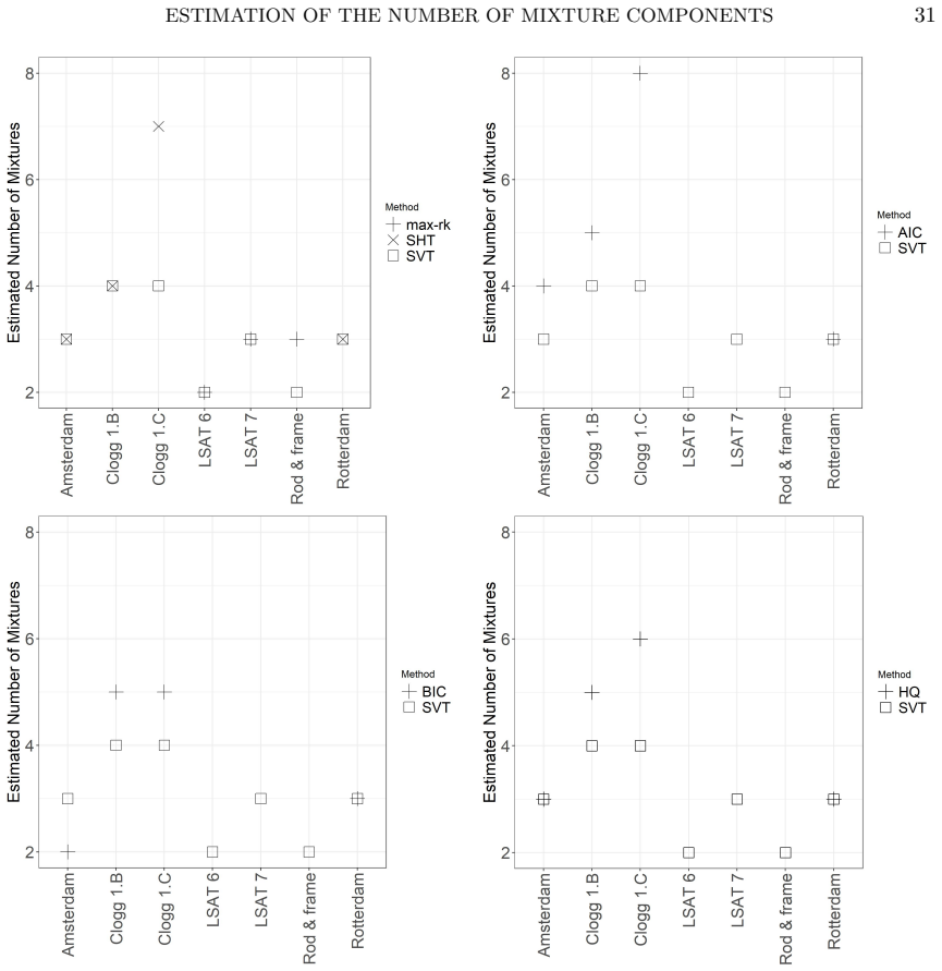
Empirical Examples. In this section, following Kasahara and Shimotsu [21], we apply our estimatorˆM on four empirical examples containing seven datasets. These datasets are obtained from Clogg [9], Van der Heijden et al. [31], Mislevy [27] and Hettmansperger and Thomas [14]. W...
[10]

and Kitamura, Y

Compiani, G. and Kitamura, Y. (2016). Using mixtures in econometric models: a brief review and some new results. Econometrics Journal 19 95-127

2016
[11]

In this paper, we introduced a novel approach for estimating the num- ber of mixture components in multivariate ﬁnite mixture models

Conclusion. In this paper, we introduced a novel approach for estimating the num- ber of mixture components in multivariate ﬁnite mixture models. Under a mild assumption on the distributions of the observed variables, we showed that the number of mixture com- ponentsM is ident...
[12]

molliﬁer

Proofs. Proof. (Proof of Proposition 2.1) By equation 1.1 T has the representation T =∑M m=1πmf 2 m⊗f 1 m. LetM1 (resp.M2) denote the subspace ofL2(S1) (respL2(S2)) spanned by the functions{f 1 m}M m=1 (resp.{f 2 m}M m=1 ). Under Assumption 2.1, the subspacesM1 and M2 have dim...
[13]

and Mira, P

Aguirregabiria, V. and Mira, P. (2019). Identiﬁcation of Games of Incomplete Informationwith Multiple Equilibria and Unobserved Heterogeneity. Quantitative Economics. 10 1659-1701

2019
[14]

, Matias, C

Allman, E. , Matias, C. and Rhodes, J. (2009). Identiﬁability of parameters in latent structure models with many observed variables. Annals of Statistics 37 3099-3132

2009
[15]

An, Y. , Hu, Y. and Shum, M. (2010). Estimating ﬁrst-price auctions with an unknown number of bidders: A misclassiﬁcation approach. Journal of Econometrics 157 328-341

2010
[16]

and Hunter, D

Benaglia, T., Chauveau, D. and Hunter, D. R. (2009). An EM-Like Algorithm for Semi- and Non- parametric Estimation in Multivariate Mixtures. Journal of Computational and Graphical Statistics 18 505-526

2009
[17]

, Bousquet, O

Blanchard, G. , Bousquet, O. and Zwald, L. (2007). Statistical Properties of Kernel Principal Component Analysis. Machine Learning 66 259-294

2007
[18]

, Jochmans, K

Bonhomme, S. , Jochmans, K. and Robin, J.-M. (2014). Nonparametric Estimation of Finite Mix- tures from Repeated Measurements. Journal of the Royal Statistical Society Series B 78 211-229

2014
[19]

, Jochmans, K

Bonhomme, S. , Jochmans, K. and Robin, J.-M. (2016). Estimating Multivariate Latent-Structure Models. Annals of Statistics 44 540-563

2016
[20]

Brezis, H. (2010). Functional Analysis, Sobolev Spaces and Partial Diﬀerential Equations . Springer- Verlag New York

2010
[21]

For the Rotterdam dataset, like our method, all their procedures estimate 3 mixture components

estimate 3, 4, 2 and 3 mixture components, using SHT, AIC, BIC and HQ, respec- tively. For the Rotterdam dataset, like our method, all their procedures estimate 3 mixture components. 5.3. Response patterns in the LSAT. Mislevy [27] studies the response patterns from of 1000 su...
[22]

Clogg, C. (1981). Latent Structure Models of Mobility. American Journal of Sociology 86 836-868

1981
[23]

and Zhou, X.-H

Hall, P. and Zhou, X.-H. (2003). Nonparametric estimation of component distributions in a multi- variate mixture. Annals of Statistics 31 201-224

2003
[24]

and Elmore, R

Hall, P., Neeman, A., Pakyari, R. and Elmore, R. (2005). Nonparametric inference in multivariate mixtures. Biometrika 92 667-678

2005
[25]

Hettmansperger, T. P. and Thomas, H. (2000a). Almost Nonparametric Inference for Repeated Measures in Mixture Models. Journal of the Royal Statistical Society. Series B (Statistical Methodol- ogy), 62 811-825

2000
[26]

Hettmansperger, T. P. and Thomas, H. (2000b). Almost Nonparametric Inference for Repeated Measures in Mixture Models. Journal of the Royal Statistical Society, Series. B 62 811-825

2000
[27]

Hoeffding, W. (1963). Probability Inequalities for Sums of Bounded Random Variables. Journal of the American Statistical Association 58 13-30

1963
[28]

and Johnson, C

Horn, R. and Johnson, C. (1991). Topics in Matrix Analysis . Cambridge University Press, Cam- bridge

1991
[29]

Hu, Y. (2008). Identiﬁcation and estimation of nonlinear models with misclassiﬁcation error using instrumental variables: A general solution. Journal of Econometrics 144 27-61

2008
[30]

, McAdams, D

Hu, Y. , McAdams, D. and Shum, M. (2013). Identiﬁcation of ﬁrst-price auctions with non-separable unobserved heterogeneity. Journal of Econometrics 174 186-193

2013
[31]

and Shum, M

Hu, Y. and Shum, M. (2012). Nonparametric identiﬁcation of dynamic models with unobserved state variables. Journal of Econometrics 171 32-44

2012
[32]

and Shimotsu, K

Kasahara, H. and Shimotsu, K. (2009). Nonparametric Identiﬁcation of Finite Mixture Models of Dynamic Discrete Choices. Econometrica 77 135-175. ESTIMATION OF THE NUMBER OF MIXTURE COMPONENTS 41

2009
[33]

and Shimotsu, K

Kasahara, H. and Shimotsu, K. (2014). Non-parametric identiﬁcation and estimation of the number of components in multivariate mixtures. Journal of the Royal Statistical Society Series B 76 97-111

2014
[34]

and Gine, E

Koltchinskii, V. and Gine, E. (2000). Random Matrix Approximation of Spectra of Integral Oper- ators. Bernoulli 6 113-167

2000
[35]

Kress, R. (1999). Linear Integral Equations. Springer, New York

1999
[36]

, Hunter, D

Levine, M. , Hunter, D. R. and Chauveau, D. (2011). Maximum smoothed likelihood for multi- variate mixtures. Biometrika 98 403-416

2011
[37]

Mbakop, E. (2017). Identiﬁcation of Auctions with Incomplete Bid Data in the Presence of Unobserved heterogeneity Working Papers, University of Calgary

2017
[38]

and Peel, D

McLachlan, G. and Peel, D. (2000). Finite Mixture Models. New York: Wiley

2000
[39]

Mislevy, R. J. (1984). Estimating Latent Distribution. Psychometrika 49 359-381

1984
[40]

Pinelis, I. (1994). Optimum Bounds for the Distributions of Martingales in Banach Spaces. Ann. Probab. 22 1679-1706

1994
[41]

and De Vito, E

Rosasco, L., Belkin, M. and De Vito, E. (2010). On Learning with Integral Operators. Journal of Machine Learning Research 11 905-934

2010
[42]

and Zhou, D.-X

Smale, S. and Zhou, D.-X. (2007). Learning Theory Estimates via Integral Operators and Their Approximations. Constructive Approximation 26 153-172

2007
[43]

van der Heijden, P. G. M. , van der Ark, L. A. and Mooijaart, A. (2002). Some Examples of Latent Budget Analysis and its Extensions. In Applied Latent Class Analysis (J. A. Hagenaars and A. L. McCutcheon, eds.) Cambridge University Press,

2002
[44]

Xiao, R. (2018). Identiﬁcation and estimation of incomplete information games with multiple equilib- ria. Journal of Econometrics 203 328-343

2018
[45]

and Blanchard, G

Zwald, L. and Blanchard, G. (2005). On the Convergence of Eigenspaces in Kernel Principal Component Analysis. In NIPS. Caleb Kwon Harvard Business School 20 N Harvard St. Boston, MA 02613 USA E-mail: calebkwon@g.harvard.edu URL: http://calebkwon.com Eric Mbakop Department of E...

2005

Pith tools

Reviewed August 14, 2026 · model on record in the stance chip above.

[1] [1]

Design 1 (mixture of 3 normal distributions): P (Θ = m) = 1 /3 for m ∈ {1, 2, 3}, and ( X1,X 2)|Θ = m ∼ N(µm,I 2), where µ1 = (0, 0)′, µ2 = (1, 2)′, µ3 = (2, 1)′, and I2 is the 2 by 2 identity matrix

work page

[2] [2]

As the Hilbert-Schmidt norm is an inner product norm, we have ‖Th,x−Th,x′‖2 HS =‖Th,x‖2 HS +‖Th,x′‖2 HS− 2⟨Th,x,Th,x′⟩HS, where⟨·,·⟩HS denotes the Hilbert-Schmidt inner product

in R2. As the Hilbert-Schmidt norm is an inner product norm, we have ‖Th,x−Th,x′‖2 HS =‖Th,x‖2 HS +‖Th,x′‖2 HS− 2⟨Th,x,Th,x′⟩HS, where⟨·,·⟩HS denotes the Hilbert-Schmidt inner product. A straightforward computation (using the deﬁnition of the Hilbert-Schmidt inner product) yields (3.26) ‖Th,x−Th,x′‖2 HS =φh(x1,x 1)φh(x2,x 2) +φh(x′ 1,x′ 1)φh(x′ 2,x′ 2)− 2...

work page

[3] [3]

approximately sharp

Estimation. In the setting of Section 2.1 ( K = 2, d1 = d2 = 1), we propose in this section an estimator of rank(T ) based on an i.i.d sample {Xi}N i=1 of X. We discuss further below (see Remark 3.5) how to extend the results to the general setting ( K >2). The main result of this section is Theorem 3.1 which provides a consistent estimator of rank(T ) of...

work page 2000

[4] [4]

In this section, we assess the performance of our estimator ˆM on ﬁve designs

Monte Carlo Experiments. In this section, we assess the performance of our estimator ˆM on ﬁve designs. The performance of ˆM is then compared to the procedures suggested by Kasahara and Shimotsu [21]: SHT, AIC, BIC, HQ (whenK = 2) and max-rk+ (whenK >2). The designs that we consider haveM = 3 andM = 5 mixture components, and for each design we simulate 1...

work page 2000

[5] [5]

Design 2 (mixture of 3 Uniform distributions): P (Θ = m) = 1/3 for m∈{ 1, 2, 3}, and (X1,X 2)|Θ = m∼U (am,bm)×U (am,bm), with am = (m− 1) and bm =m

work page

[6] [6]

Design 3 (mixture of 3 normal distributions): P (Θ = m) = 1 /3 for m ∈ {1, 2, 3}, and ( X1,X 2)|Θ = m ∼ N(µm,I 2), where µ1 = (0, 0)′, µ2 = (3, 3)′, µ3 = (−3,−3)′, and I2 is the 2 by 2 identity matrix

work page

[7] [7]

Design 4 (mixture of 5 uniform distributions): P (Θ = m) = 1 /5 for m ∈ {1, 2, 3, 4, 5}, and ( X1,X 2)|Θ = m ∼ U(am,bm)× U(am,bm), with am = (m− 1) and bm =m

work page

[8] [8]

irregular

Design 5 (mixture of 3 normal distributions): P (Θ =m) = 1/3 for m∈{ 1, 2, 3}, and (X1,X 2,··· ,X 8)|Θ = m∼N (µm,I 8), where with µ1 = (0, 0, 0, 0, 0, 0, 0, 0)′,µ 2 = (1.0, 2.0, 0.5, 1.0, 0.75, 1.25, 0.25, 0.5)′,µ 3 = (2.0, 1.0, 1.0, 0.5, 1.25, 0.75, 0.5, 0.25)′, and I8 is the 8 by 8 identity matrix. The outcome of the simulations are presented in the tab...

work page 2000