REVIEW 2 major objections 7 minor 54 references
Lagrangian Dynamic Mode Decomposition for Construction of Reduced-Order Models of Advection-Dominated Phenomena
T0 review · 2 major / 7 minor · reviewed 2026-08-14 · deepseek-v4-flash
Pith's one-line read This paper claims that running DMD on the Lagrangian observable $(x,u)$, where $x$ tracks moving characteristic lines, builds reduced-order models that stay accurate beyond the training window for shock-free advection-dominated problems.
desk verdict A genuinely useful incremental extension of Lagrangian POD to DMD, with clean shock-free tests—but the crucial Eulerian-only-data route for getting characteristic trajectories is never demonstrated, so its central promise outruns its evidence. read the letter →
The pith
A machine-rendered reading of the paper's core claim, the machinery that carries it, and where it could break.
The reading
What carries the argument
The load-bearing object is the observable vector $y^n=(x^n,u^n)$ built from the semi-Lagrangian formulation of the advection-diffusion equation, which tracks characteristic lines through the ordinary differential equation $dX/dt=f(u(X(t),t))$. The DMD algorithm approximates the Koopman operator, the infinite-dimensional linear operator that advances observable functions of the state, restricted to the invariant subspace spanned by these observables under Assumption 3.1. The characteristic-line positions are what do the work: they translate the moving wave into a frame in which the low-rank SVD basis does not have to chase the signal, which is exactly the failure mode diagnosed for Eulerian DMD in Section 2.3.
What would settle it
Run the same Lagrangian-DMD pipeline on a problem in which characteristic lines cross, such as inviscid Burgers evolved past the shock-formation time, and record the global truncation error $E^n$; the central claim would be falsified if the error stops following the Theorem 4.1 bound and grows without control or produces unphysical oscillations, since the paper's own conclusion states that all its tests are shock-free and that the Lagrangian grid may entangle.
Extended reading notes
Core claim
The paper's central discovery is that the translational difficulty of advection-dominated flows is a coordinate problem, not a fundamental limit of DMD or POD. By choosing the observable $y^n=(x^n,u^n)$, the vector of characteristic-line positions together with solution values on those lines, the authors obtain a finite-dimensional Koopman-invariant subspace in which the moving wave is stationary relative to the basis. The DMD algorithm (Algorithm 3.1) then approximates the Koopman operator restricted to this subspace, and future states are predicted analytically by $y^n=\Phi \Lambda^n b$. In the tested shock-free regimes the resulting ROM remains accurate in the extrapolating mode, i.e., for $t>0.25$, and the error bound of Theorem 4.1 gives a computable estimate of how long that accuracy lasts.
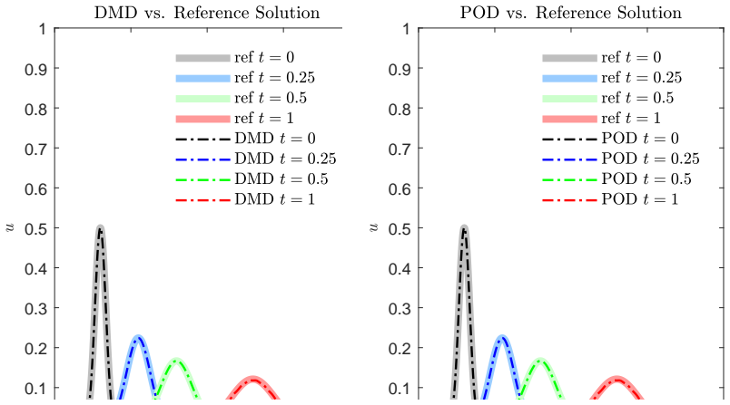
Load-bearing premise
The load-bearing premise is that a small set of fixed modes can exactly represent the coupled motion of the moving grid positions and the solution values on them, and that the training data reliably supply those moving grid positions; the tests obtain them from a Lagrangian solver, so the method's success depends on that supply.
Editorial extensions
If this is right
- For shock-free advection-dominated problems, a single low-rank basis constructed on $(x,u)$ extrapolates accurately far beyond the training window $t\le 0.25$, where Eulerian DMD and POD fail.
- Because future states come from one direct evaluation of the prediction formula, Lagrangian DMD requires no iteration in the low-dimensional space, making it the cheapest ROM among those compared while matching Lagrangian POD's accuracy in most tests.
- The error bound in Theorem 4.1 provides an a priori estimate of the observable's error, allowing one to design a hybrid scheme that runs the high-fidelity model for a short time and then switches to the ROM for long-time prediction.
- The level-set experiment in the appendix shows that the same Lagrangian-observable idea can be applied to conservation laws by reformulating them as two-dimensional linear transport, capturing the inviscid Burgers solution at rank $r=3$.
Reading between the lines
- If characteristic positions can be recovered from Eulerian-only data by tracking wave crests, level sets, or feature velocities, the same ROM construction should work without a dedicated Lagrangian solver; the paper outlines this route in Section 3.1 but does not test it, so this remains an inference about an untested extension.
- SVD-based ROMs for moving fronts have usually been repaired with local bases, domain decomposition, or multiresolution filtering; the Lagrangian-observable choice suggests a single global basis can suffice for a wider class of problems, provided the characteristic grid does not entangle.
- A natural stress test beyond the four textbook cases is to add small noise or slightly random initial conditions and watch whether the Koopman-invariant-subspace assumption degrades gracefully; the paper does not report such a test, so the practical robustness of the extrapolating mode is still open.
Signed reviews
Editorial analysis
A structured set of objections, weighed in public.
Referee Report
Summary. The manuscript proposes a Lagrangian reformulation of dynamic mode decomposition for reduced-order modeling of advection-dominated PDEs. It first demonstrates with a linear advection example that standard Eulerian POD and DMD generate global SVD bases that cannot represent a translating pulse, leading to inaccurate extrapolation. It then introduces Algorithm 3.1, which applies the standard DMD procedure to the augmented observable y^n = [x^n; u^n], where x^n denotes characteristic-line positions, and reconstructs u from the predicted observable. Numerical experiments on linear advection, linear advection-diffusion, inviscid and viscous Burgers equations, and a level-set formulation are presented; all reported tests are shock-free. In these tests, Lagrangian DMD and Lagrangian POD capture the solution beyond the training window t > 0.25, with DMD being cheaper because it is iteration-free. An error bound from a previous paper by the same authors is quoted and plotted.
Significance. Should the method hold, it offers a simple physics-aware extension of DMD that is equation-free and iteration-free and that directly addresses the translation failure of Eulerian SVD methods. The choice of [x; u] as observables is physically motivated and is not tuned to the test outputs. The numerical comparisons against conventional Eulerian DMD and POD are clean and convincing for the shock-free cases. The main caveat is that the method's success depends on the availability of accurate characteristic trajectories; this dependence is acknowledged only indirectly and is not validated in the standard Eulerian-snapshot data regime. Given the explicit shock-free limitation and the unvalidated data pipeline, the contribution is promising but not yet established at the claimed scope.
major comments (2)
- [Section 4 / Table 1] The numerical validation supplies the characteristic positions x^n from a separate Lagrangian high-fidelity solve, as the listing of 'Lagrangian HFM computational time' in Table 1 indicates, rather than deriving them from the Eulerian reference snapshots produced by (2.3). For an end user with Eulerian-only data, the route described in Section 3.1 is stated only for Lagrangian POD (following [30, Sec. 3.3]) and is neither formulated nor tested for Lagrangian DMD. Because Algorithm 3.1 requires x^n as an observable, this is a load-bearing gap: if characteristic trajectories cannot be recovered accurately from the available data, the method's advantage disappears. The authors should either demonstrate trajectory recovery from Eulerian snapshots and use it in the numerical tests, or explicitly restrict the paper's claim to settings in which Lagrangian trajectory data are available.
- [Theorem 4.1] The error bound used in every numerical example is quoted from [20], but epsilon_m is not defined in this manuscript and the theorem is stated without proof or a precise pointer to the statement in [20]. Since the figures plot this bound as an estimate of the observable error, a reader cannot verify whether the plotted curve is actually the right-hand side of (4.2). The authors should either include the definition of epsilon_m and the main steps of the proof, or remove the bound from the figures and state the error analysis as a reference.
minor comments (7)
- [Algorithm 3.1, Step 2] The matrix X' should be Y2; as written, the low-rank approximation K-tilde is not defined in terms of the observable data matrices introduced in Step 0.
- [Eqs. (2.17) and (3.9)] The prediction formulas use Lambda^{n+1} with b = Phi^{-1} y^1 (or u^0), but the standard DMD convention with snapshots indexed from 1 gives y^n = Phi Lambda^{n-1} b. Please clarify the indexing so the extrapolation formula is unambiguous.
- [Figure 7 caption] The caption says 'linear advection equation,' but Section 4.2 concerns the linear advection-diffusion equation; please correct.
- [Abstract and Introduction] The conclusion explicitly states that all tests are shock-free, but the abstract and introduction do not carry this qualification; readers may overinterpret the scope. Please state the shock-free limitation prominently in the abstract.
- [Sections 3.1 and 3.2] The phrases 'optimal Lagrangian basis' and 'optimal choice of observable functions' are not backed by an optimality criterion; 'well-motivated' or 'physics-informed' would be more accurate.
- [Appendix A] The level-set DMD experiment would benefit from a precise statement of the observable matrix, the number of snapshots, the SVD rank, and the reconstruction procedure to be reproducible.
- [Section 1] There are several typos, e.g., 'explaination' and 'physic-aware'; a careful proofreading pass is needed.
Circularity Check
No circular derivation: Lagrangian DMD is a standard Koopman/DMD fit on an augmented observable with extrapolative tests; the sole self-citation (error bound from companion paper) is not load-bearing.
full rationale
The claimed prediction is extrapolation beyond the training window (m=250 snapshots, t<=0.25; error plots extend to t=1), so it is not a fitted input renamed as a prediction. The observable y=[x;u] (Eq. 3.11) is chosen from the physics of characteristics before fitting and is not optimized against the test outputs. The DMD algorithm (Algorithm 3.1) is the standard linear least-squares fit on snapshots; no equation in the paper defines the observable in terms of the predicted quantity or fits a parameter to the validation data. The paper's acknowledged reliance on Lagrangian-solver-generated trajectories, and its untested Eulerian-only-data route (Section 3.1), is a limitation of data availability, not a circular reduction. Theorem 4.1 is a bound from the authors' companion paper [20]; it is used only to plot an error estimate and is not needed to build the ROM, so it is a minor self-citation but not load-bearing. No significant circularity.
Assumptions & free parameters
free parameters (2)
- SVD rank truncation r (energy threshold epsilon) =
r = 3, 10, 3, 14 for Tests 1-4; epsilon = 1e-8 in Section 4, 1e-4 in Section 2
- Number of training snapshots m =
m = 250 for all Lagrangian tests
assumptions (4)
- domain assumption Assumption 3.1: the chosen observable vector y=(x,u) lies in a finite-dimensional Koopman-invariant subspace; otherwise the finite DMD representation is not valid.
- domain assumption The semi-Lagrangian discretization (3.1)-(3.2) accurately tracks characteristic lines and interpolation between grids is stable.
- domain assumption All test problems are shock-free within the prediction horizon, so characteristic lines do not cross and the Lagrangian formulation remains valid.
- standard math Error bound in Theorem 4.1, taken from the authors' companion paper [20], is correct.
Cite this review
Pith. "Pith review of Lagrangian Dynamic Mode Decomposition for Construction of Reduced-Order Models of Advection-Dominated Phenomena." pith.science (2026). https://pith.science/paper/FVKBU46B
@misc{pith2026190803688,
  author       = {Pith},
  title        = {Pith review of: Lagrangian Dynamic Mode Decomposition for Construction of Reduced-Order Models of Advection-Dominated Phenomena},
  year         = {2026},
  howpublished = {\url{https://pith.science/paper/FVKBU46B}},
  note         = {Machine review of arXiv:1908.03688}
}
read the original abstract
Proper orthogonal decomposition (POD) and dynamic mode decomposition (DMD) are two complementary singular-value decomposition (SVD) techniques that are widely used to construct reduced-order models (ROMs) in a variety of fields of science and engineering. Despite their popularity, both DMD and POD struggle to formulate accurate ROMs for advection-dominated problems because of the nature of SVD-based methods. We investigate this shortcoming of conventional POD and DMD methods formulated within the Eulerian framework. Then we propose a Lagrangian-based DMD method to overcome this so-called translational issues. Our approach is consistent with the spirit of physics-aware DMD since it accounts for the evolution of characteristic lines. Several numerical tests are presented to demonstrate the accuracy and efficiency of the proposed Lagrangian DMD method.
Figures


Figures from the paper (9 more)




Reference graph
Works this paper leans on
- [20]
-
[1]
Introduction Advection-diffusion equations are routinely used as a high-fidelity re presentation of mass conservation at a variety of spatiotemporal scales in a plethora of applications [1]. These equations become highly nonlinear when advection velocity and/or diffusion coefficient depend (s) on a system state, e.g., in the case of multiphase flows in porous m...
work page 2019
-
[2]
Conventional Eulerian Reduced-Order Models Consider a scalar state variable u(x, t ) : [ a, b ] × [0, T ] → R+, whose dynamics is described by a one-dimensional nonlinear advection-diffusion equation ∂u ∂t + f (u) ∂u ∂x = ∂ ∂x ( D(x, t, u ) ∂u ∂x ) , f (u) = ∂F (u) ∂u , (2.1) subject to the initial condition u(x, t = 0) = u0(x) (2.2) and appropriate (arbit...
- [3]
-
[4]
Compute ˜K = U∗X2VΣ −1 as an r × r low-rank approximation of K
-
[5]
Compute eigendecomposition of ˜K: ˜KW = WΛ , Λ = (λ k). 5
-
[6]
Each column of Φ is a DMD mode corresponding to a particular eigenvalue in Λ
Reconstruct eigendecomposition of K, whose eigenvalues and eigenvectors are Λ and Φ = UW, respectively. Each column of Φ is a DMD mode corresponding to a particular eigenvalue in Λ . With the ap- proximated eigenvalues and eigenvectors of K in hand, the projected future solution can be constructed analytically for all times in the future. In particular, a...
work page 2000
-
[7]
Lagrangian Reduced-Order Models Motivated by construction of a POD-based ROM for the advection- diffusion equation (2.1) within the Lagrangian framework [30], we propose a Lagrangian DMD. In th e semi-Lagrangian frame, (2.1) is written as dX(t) dt = f (u(X(t), t )), du(x, t ) dt ⏐ ⏐ ⏐ ⏐ x=X(t) = [ ∂ ∂x ( D(x, t, u ) ∂u(x, t ) ∂x )] ⏐ ⏐ ⏐ ⏐ x=...
Show all 54 references
-
[8]
Create data matrices of observables Y1 and Y2 as Y1 = | | | y1 y2 · · · ym−1 | | | , Y2 = | | | y2 y3 · · · ym | | | , (3.8) where each column is given by yk = g(uk).135
-
[9]
Compute SVD of the matrix Y1 ≈ UΣV ∗ with U ∈ Cp×r, Σ ∈ Rr×r, V ∈ Cr×m, where r is the truncated rank chosen by certain criteria
-
[10]
Compute ˜K = U∗X′VΣ −1 as an r × r low-rank approximation for K
-
[11]
Compute eigendecomposition of ˜K: ˜KW = WΛ , Λ = (λ k)
-
[12]
Eigenvalues are Λ and eigenvectors are Φ = UW.140 11
Reconstruct eigendecomposition of K. Eigenvalues are Λ and eigenvectors are Φ = UW.140 11
-
[13]
Future yn+1 DMD can be predicted by yn+1 DMD = ΦΛ n+1b, n > m (3.9) with b = Φ −1y1
-
[14]
(3.10) In data-driven modeling, judicious selection of the observables is cr ucial to the accuracy and efficiency of a Koopman operator’s approximation
Transform from observables back to state-space: un DMD = g−1(yn DMD). (3.10) In data-driven modeling, judicious selection of the observables is cr ucial to the accuracy and efficiency of a Koopman operator’s approximation. Identification of general rules for choosing the observab...
-
[15]
In all tests, the reference solutions are145 computed in the Eulerian framework using (2.3)
Numerical Experiments To ascertain the accuracy and robustness of the Lagrangian DMD , we use it to construct ROMs for a series of linear and nonlinear advection-dominated problems. In all tests, the reference solutions are145 computed in the Eulerian framework using (2.3). Th...
2000
-
[16]
05 )2] (4.3a) and boundary conditions u(0, t ) = u(2, t ) = 0 . (4.3b) 0 0.5 1 1.5 2 0 0.1 0.2 0.3 0.4 0.5 0.6 0.7 0.8 0.9 1 0 0.5 1 1.5 2 0 0.1 0.2 0.3 0.4 0.5 0.6 0.7 0.8 0.9 1 Figure 4: Solutions of the linear advection equation, u(x, t), alternatively obtained with the num...
-
[17]
A new physic-aware DMD, based on the Lagrangian framework, is propos ed to overcome the shortcomings of reduced order models (ROMs) of advection-dominated nonlinear phenomena
Conclusions200 In this paper, we investigate the issue of translational problem for conventional proper orthogonal decomposition (POD) and dynamic mode decomposition (DMD) in the Eu lerian framework. A new physic-aware DMD, based on the Lagrangian framework, is propos ed to ov...
-
[18]
D. Duke, J. Soria, D. Honnery, An error analysis of the dynamic mode decomposition, Exper. Fluids275 52 (2) (2012) 529–542
2012
-
[19]
D. M. Tartakovsky, M. Dentz, Diffusion in porous media: Phenome na and mechanisms, Transp. Porous Media (2019). doi:10.1007/s11242-019-01262-6 .240
2019 doi
-
[21]
Quarteroni, G
A. Quarteroni, G. Rozza, et al., Reduced order methods for mod eling and computational reduction, Vol. 9, Springer, 2014
2014
-
[22]
Acharjee, N
S. Acharjee, N. Zabaras, A concurrent model reduction appr oach on spatial and random domains245 for the solution of stochastic PDEs, Int. J. Num. Meth. Engrg. 66 (12) (2006) 1934–1954
2006
-
[23]
Holmes, J
P. Holmes, J. L. Lumley, G. Berkooz, C. W. Rowley, Turbulence, c oherent structures, dynamical systems and symmetry, Cambridge Univ. Press, 2012
2012
-
[24]
J. L. Lumley, Stochastic tools in turbulence, Courier Corporatio n, 2007
2007
-
[25]
Volkwein, Model reduction using proper orthogonal decompo sition, Lecture Notes, Insti-250 tute of Mathematics and Scientific Computing, University of Graz
S. Volkwein, Model reduction using proper orthogonal decompo sition, Lecture Notes, Insti-250 tute of Mathematics and Scientific Computing, University of Graz. s ee http://www. uni-graz. at/imawww/volkwein/POD. pdf 1025 (2011)
2011
-
[26]
Barrault, Y
M. Barrault, Y. Maday, N. C. Nguyen, A. T. Patera, An empirical interpolation method: application to efficient reduced-basis discretization of partial differential equ ations, Comptes Rendus Mathema- tique 339 (9) (2004) 667–672.255
2004
-
[27]
Chaturantabut, D
S. Chaturantabut, D. C. Sorensen, Nonlinear model reduction via discrete empirical interpolation, SIAM J. Sci. Comput. 32 (5) (2010) 2737–2764
2010
-
[28]
J. N. Kutz, S. L. Brunton, B. W. Brunton, J. L. Proctor, Dyn amic mode decomposition: data-driven modeling of complex systems, Vol. 149, SIAM, 2016
2016
-
[29]
Mezi´ c, Analysis of fluid flows via spectral properties of the Koopman operator, Annu
I. Mezi´ c, Analysis of fluid flows via spectral properties of the Koopman operator, Annu. Rev. Fluid260 Mech. 45 (2013) 357–378
2013
-
[30]
B. O. Koopman, Hamiltonian systems and transformation in Hilber t space, Proc. Natl. Acad. Sci. U.S.A. 17 (5) (1931) 315
1931
-
[31]
Mezi´ c, Spectral properties of dynamical systems, mode l reduction and decompositions, Nonlin
I. Mezi´ c, Spectral properties of dynamical systems, mode l reduction and decompositions, Nonlin. Dyn. 41 (1-3) (2005) 309–325.265 21
2005
-
[32]
bypass this issue by compensating computational costs in proj ecting back to the Eulerian grid. From the perspective of physic-aware data-driven modeling, we realize t hat significant information like shock220 formation time, shock location and shock speed is not interpreted w ...
-
[33]
Mezi´ c, A
I. Mezi´ c, A. Banaszuk, Comparison of systems with complex b ehavior, Physica D 197 (1-2) (2004) 101–133
2004
-
[34]
C. W. Rowley, I. Mezi´ c, S. Bagheri, P. Schlatter, D. S. Hennin gson, Spectral analysis of nonlinear flows, J. Fluid Mech. 641 (2009) 115–127
2009
-
[35]
S. L. Brunton, J. L. Proctor, J. N. Kutz, Discovering govern ing equations from data by sparse270 identification of nonlinear dynamical systems, Proc. Natl. Acad. Sc i. U.S.A. 113 (15) (2016) 3932– 3937
2016
-
[36]
Schmidt, H
M. Schmidt, H. Lipson, Distilling free-form natural laws from exp erimental data, Science 324 (5923) (2009) 81–85
2009
-
[37]
Korda, I
M. Korda, I. Mezi´ c, On convergence of extended dynamic mo de decomposition to the Koopman operator, J. Nonlin. Sci. 28 (2) (2018) 687–710
2018
-
[38]
H. Lu, D. M. Tartakovsky, Prediction accuracy analysis for dy namic mode decomposition, ArXiv (2019).280
2019
-
[39]
Amsallem, M
D. Amsallem, M. J. Zahr, C. Farhat, Nonlinear model order redu ction based on local reduced-order bases, Int. J. Num. Meth. Engrg. 92 (10) (2012) 891–916
2012
-
[40]
D. J. Lucia, Reduced order modeling for high speed flows with mov ing shocks, Tech. rep., Air Force Inst. of Tech., Wright-Patterson Air Force Base, OH (2001)
2001
-
[41]
Carlberg, Adaptive h-refinement for reduced-order mode ls, Int
K. Carlberg, Adaptive h-refinement for reduced-order mode ls, Int. J. Num. Meth. Engrg. 102 (5)285 (2015) 1192–1210
2015
-
[42]
J. N. Kutz, X. Fu, S. L. Brunton, Multiresolution dynamic mode d ecomposition, SIAM J. Appl. Dyn. Syst. 15 (2) (2016) 713–735
2016
-
[43]
Gerbeau, D
J.-F. Gerbeau, D. Lombardi, Approximated Lax pairs for the re duced order integration of nonlinear evolution equations, J. Comput. Phys. 265 (2014) 246–269.290
2014
-
[44]
M. E. Kavousanakis, R. Erban, A. G. Boudouvis, C. W. Gear, I. G. Kevrekidis, Projective and coarse projective integration for problems with continuous symme tries, J. Comput. Phys. 225 (1) (2007) 382–407
2007
-
[45]
Rap´ un, J
M.-L. Rap´ un, J. M. Vega, Reduced order models based on local POD plus Galerkin projection, J. Comput. Phys. 229 (8) (2010) 3046–3063.295 22
2010
-
[46]
C. W. Rowley, I. G. Kevrekidis, J. E. Marsden, K. Lust, Reduct ion and reconstruction for self-similar dynamical systems, Nonlinearity 16 (4) (2003) 1257
2003
-
[47]
C. W. Rowley, J. E. Marsden, Reconstruction equations and th e Karhunen–Lo` eve expansion for systems with symmetry, Physica D 142 (1-2) (2000) 1–19
2000
-
[48]
Mojgani, M
R. Mojgani, M. Balajewicz, Lagrangian basis method for dimensio nality reduction of convection300 dominated nonlinear flows, arXiv preprint arXiv:1701.04343 (2017)
2017 arXiv
-
[49]
S. L. Brunton, B. W. Brunton, J. L. Proctor, J. N. Kutz, Koo pman invariant subspaces and finite linear representations of nonlinear dynamical systems for contro l, PloS One 11 (2) (2016) e0150171
2016
-
[50]
Morton, A
J. Morton, A. Jameson, M. J. Kochenderfer, F. Witherden, D eep dynamical modeling and control of unsteady fluid flows, in: Advances in Neural Information Processin g Systems, 2018, pp. 9278–9288.305
2018
-
[51]
Thiffeault, Advection-diffusion in Lagrangian coordinates, Phys
J.-L. Thiffeault, Advection-diffusion in Lagrangian coordinates, Phys. Lett. A 309 (5-6) (2003) 415– 422
2003
-
[52]
Shashkov, B
M. Shashkov, B. Wendroff, A composite scheme for gas dynamic s in Lagrangian coordinates, J. Comput. Phys. 150 (2) (1999) 502–517
1999
-
[53]
S. E. Hieber, P. Koumoutsakos, A Lagrangian particle level set method, Journal of Computational310 Physics 210 (1) (2005) 342–367
2005
-
[54]
Y.-H. Tsai, Y. Giga, S. Osher, A level set approach for computin g discontinuous solutions of Hamilton-Jacobi equations, Math. Comput. 72 (241) (2003) 159– 181. 23
2003
Reviewed August 14, 2026 · model on record in the stance chip above.
Discussion (0). Continue with ORCID to comment.