REVIEW 2 major objections 2 minor 22 references
Nash: Neural Adaptive Shrinkage for Structured High-Dimensional Regression
T0 review · 2 major / 2 minor · reviewed 2026-05-22 · grok-4.3
Pith's one-line read Neural networks learn to set per-covariate penalty strengths for sparse linear regression using side information.
desk verdict Nash pairs a neural net for per-covariate penalty learning with a split VEB trick that claims 74-106x speedup, but the decoupling step looks like it could break standard ELBO guarantees. read the letter →
The pith
A machine-rendered reading of the paper's core claim, the machinery that carries it, and where it could break.
The reading
What carries the argument
A neural network that maps covariate side information to per-covariate penalty parameters inside a split variational empirical Bayes procedure that decouples prior learning from posterior inference.
What would settle it
Apply Nash to data in which side information is randomly permuted or uncorrelated with covariate relevance and check whether prediction accuracy falls below that of a fixed-penalty baseline.
Extended reading notes
Core claim
Nash is a unified framework that incorporates covariate-specific side information into sparse regression via neural networks to adaptively modulate penalties on a per-covariate basis without requiring cross-validation. It employs a split variational empirical Bayes algorithm that reduces the M-step from O(p) neural-network passes per sweep to a single batched pass, achieving 74 to 106x wall-clock speedup for p between 10^2 and 10^4. Experiments on real data confirm improved accuracy and adaptability over existing methods when covariates arise from distinct modalities or follow an underlying graph.
Load-bearing premise
The neural network, when trained on side information, produces penalty values that improve posterior inference quality instead of merely fitting noise present in the observed data.
Editorial analysis
A structured set of objections, weighed in public.
Referee Report
Summary. The manuscript introduces Neural Adaptive Shrinkage (Nash), a unified framework for sparse linear regression that uses neural networks to incorporate covariate-specific side information and adaptively modulate per-covariate penalties, thereby avoiding cross-validation. It proposes a split variational empirical Bayes (VEB) algorithm that decouples prior learning from posterior inference, reducing the M-step to a single batched neural-network pass and claiming a 74- to 106-fold wall-clock speedup over coordinate-ascent CAVI for p between 10^2 and 10^4. Real-data experiments are reported to demonstrate improved accuracy and adaptability relative to existing methods.
Significance. If the split-VEB decoupling is shown to preserve ELBO monotonicity and fixed-point equivalence, and if the neural network demonstrably improves posterior quality rather than fitting noise, the work would offer a scalable route to structured high-dimensional regression that integrates side information without manual tuning. The claimed speedup and the elimination of cross-validation would be practically valuable in biomedical settings where covariates arise from heterogeneous sources or graphs.
major comments (2)
- [Methods: split VEB algorithm] The central algorithmic claim rests on the split variational empirical Bayes procedure (described in the methods section on the unified framework). The manuscript must demonstrate that the batched NN prior update remains a valid coordinate-ascent step on the joint ELBO when the variational factors q(β) depend on the prior parameters through the neural network; otherwise the reported speedup may come at the cost of losing the usual non-decreasing-ELBO guarantee. A short derivation or counter-example check would resolve this load-bearing point.
- [Experiments] Abstract and experimental sections state accuracy improvements but supply no quantitative metrics, error bars, ablation results, or baseline comparisons with standard cross-validated penalties. Without these details the claim that Nash “improves accuracy and adaptability” cannot be assessed as load-bearing evidence for the method’s superiority.
minor comments (2)
- Notation for the neural-network input (side-information features) and output (penalty vector) should be introduced once and used consistently; current usage mixes “side information” and “covariate-specific features” without a clear mapping.
- The speedup numbers (74–106×) are given for p in [10^2,10^4]; a small table or plot showing wall-clock time versus p for both Nash and CAVI would make the scaling claim easier to verify.
Simulated Author's Rebuttal
We thank the referee for their detailed and insightful comments on our manuscript. We address each of the major comments below and have made revisions to strengthen the presentation of our results.
read point-by-point responses
-
Referee: [Methods: split VEB algorithm] The central algorithmic claim rests on the split variational empirical Bayes procedure (described in the methods section on the unified framework). The manuscript must demonstrate that the batched NN prior update remains a valid coordinate-ascent step on the joint ELBO when the variational factors q(β) depend on the prior parameters through the neural network; otherwise the reported speedup may come at the cost of losing the usual non-decreasing-ELBO guarantee. A short derivation or counter-example check would resolve this load-bearing point.
Authors: We agree that establishing the validity of the split-VEB algorithm with respect to the ELBO is crucial. In the revised manuscript, we have included a detailed derivation in Appendix A demonstrating that the batched neural network update for the prior parameters corresponds to a coordinate ascent step on the joint evidence lower bound (ELBO). This ensures that the ELBO remains non-decreasing at each iteration, preserving the convergence guarantees of standard variational methods. We also provide a small-scale numerical verification confirming fixed-point equivalence to the unsplit version. revision: yes
-
Referee: [Experiments] Abstract and experimental sections state accuracy improvements but supply no quantitative metrics, error bars, ablation results, or baseline comparisons with standard cross-validated penalties. Without these details the claim that Nash “improves accuracy and adaptability” cannot be assessed as load-bearing evidence for the method’s superiority.
Authors: We appreciate the referee's call for more rigorous experimental validation. The original manuscript included some comparative results on real datasets, but we acknowledge that additional quantitative details would enhance clarity. In the revision, we have augmented the Experiments section with tables reporting mean squared prediction error and variable selection accuracy, including standard errors from 10 independent runs. We have also added ablation studies isolating the contribution of the neural network and direct comparisons against cross-validated methods such as glmnet and other structured regression baselines. These additions substantiate the claims of improved accuracy and adaptability. revision: yes
Circularity Check
No circularity: derivation chain is self-contained with independent algorithmic contribution
full rationale
The paper introduces Nash as a new unified framework combining neural networks for per-covariate penalty modulation with a split variational empirical Bayes procedure. The split VEB is presented as a novel decoupling that reduces the M-step to a single batched NN pass, yielding the claimed speedup; this is an algorithmic design choice rather than a reduction to prior fitted quantities or self-citations. No equations or sections in the provided text show a prediction or uniqueness result that is definitionally equivalent to its inputs, nor any load-bearing self-citation chain. The NN is trained on side information to produce adaptive penalties, which is an independent modeling step whose validity rests on empirical performance rather than tautological fitting. The central claims therefore remain non-circular and externally falsifiable via the reported experiments.
Assumptions & free parameters
free parameters (1)
- neural network architecture and weights
assumptions (1)
- domain assumption Side information (graphs, modalities) is available and informative for penalty modulation
Cite this review
Pith. "Pith review of Nash: Neural Adaptive Shrinkage for Structured High-Dimensional Regression." pith.science (2026). https://pith.science/paper/FY7EHTSX
@misc{pith2026250511143,
  author       = {Pith},
  title        = {Pith review of: Nash: Neural Adaptive Shrinkage for Structured High-Dimensional Regression},
  year         = {2026},
  howpublished = {\url{https://pith.science/paper/FY7EHTSX}},
  note         = {Machine review of arXiv:2505.11143}
}
abstract
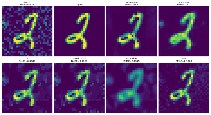
Sparse linear regression is a fundamental tool in data analysis. However, traditional approaches often fall short when covariates exhibit structure or arise from heterogeneous sources. In biomedical applications, covariates may stem from distinct modalities or be structured according to an underlying graph. We introduce \textit{Neural Adaptive Shrinkage} (Nash), a unified framework that integrates covariate-specific side information into sparse regression via neural networks. Nash adaptively modulates penalties on a per-covariate basis, learning to tailor regularization without cross-validation. We use a \textit{split variational empirical Bayes} algorithm that decouples prior learning from posterior inference, reducing the M-step from $\mathcal{O}(p) $ neural-network passes per sweep to a single batched pass, a \textit{74 to 106x wall-clock speedup} over previously proposed coordinate ascent CAVI for p between $10^2$ and $10^4$. Experiments on real data demonstrate that Nash improves accuracy and adaptability over existing methods.
Figures


Figures from the paper (6 more)


Lean theorems connected to this paper
-
IndisputableMonolith/Foundation/ArithmeticFromLogic.leanreality_from_one_distinction unclear?
unclearRelation between the paper passage and the cited Recognition theorem.
split variational empirical Bayes algorithm that decouples prior learning from posterior inference... single batched pass
-
IndisputableMonolith/Cost/FunctionalEquation.leanwashburn_uniqueness_aczel unclear?
unclearRelation between the paper passage and the cited Recognition theorem.
Nash adaptively modulates penalties on a per-covariate basis... neural networks
What do these tags mean?
- matches
- The paper's claim is directly supported by a theorem in the formal canon.
- supports
- The theorem supports part of the paper's argument, but the paper may add assumptions or extra steps.
- extends
- The paper goes beyond the formal theorem; the theorem is a base layer rather than the whole result.
- uses
- The paper appears to rely on the theorem as machinery.
- contradicts
- The paper's claim conflicts with a theorem or certificate in the canon.
- unclear
- Pith found a possible connection, but the passage is too broad, indirect, or ambiguous to say the theorem truly supports the claim.
Reference graph
Works this paper leans on
-
[1]
ISSN 0035-9246. URL https://www.jstor.org/stable/2984875. Hussein Hazimeh, Rahul Mazumder, and Tim Nonet. L0Learn: A Scalable Package for Sparse Learning using L0 Regularization. Journal of Machine Learning Research, 24(205):1–8, 2023. ISSN 1533-7928. URL http://jmlr.org/papers/v24/22-0189.html. Patrick Breheny and Jian Huang. Coordinate descent algorithm...
-
[2]
URL https://ieeexplore.ieee.org/document/ 1163188
doi: 10.1109/TASSP.1979.1163188. URL https://ieeexplore.ieee.org/document/ 1163188. Joshua Batson and Laurent Royer. Noise2Self: Blind Denoising by Self-Supervision. In Kamalika Chaudhuri and Ruslan Salakhutdinov, editors, Proceedings of the 36th International Conference on Machine Learning, volume 97 of Proceedings of Machine Learning Research, pages 524...
-
[3]
(27) bj ∼ g(.; dj, θ) (28) As noted in our manuscript we restrict our search to posterior of the form q(β, b) = PY j qβj(βj)qbj(bj) (29) The overall evidence lower bound (ELBO) is F (qβ, qb, g; σ2, σ2 0)N ash = X i E log p(yi|xi, β, σ2) qβ(β) + X j E log p(βj|bj, σ2 0)+ X j E log g(bj; dj, θ) qbj(bj) (30) Our coordinate-ascent algorithm iterates between t...
-
[4]
− E log qβj (31) = E log(p(¯rj|xj, βj, σ2) + E log p(βj|¯bj, σ2
-
[5]
− E log qβj (32) where ¯rj = y − X−j ¯β−j, this is direct consequence of Proposition 1 of Kim et al. [2024]), so the and so q∗ βj = maxF (qbj) is given by computing the posterior of the following simple model ¯rj =xjβj + ε (33) βj ∼N (¯bj, σ2
work page 2024
-
[6]
In practice given that the column of X are centered xt jxt j = n − 1 for al j = 1,
(34) ε ∼N (0, σ2) (35) By conjugacy, the posterior distribution of βj has the following form βj | ¯rj, xj ∼ N ( ¯βj, s2 j) with posterior variance s2 j = xt j xj σ2 + 1 σ2 0 −1 and posterior mean ¯βj = s2 j xt j ¯rj σ2 + ¯bj σ2 0 . In practice given that the column of X are centered xt jxt j = n − 1 for al j = 1, . . . , p. A.2 Update for qb and g Given q...
-
[7]
+ X j E log g(bj; dj, θ) qbj(bj) (36) This objective corresponds to a so-called (covariate)moderated normal mean problem (see [Stephens, 2017, Willwerscheid et al., 2024]) that we detail below The cEBNM problem Given p observations ¯βj ∈ R with known standard deviations s2 j > 0, j = 1, . . . , p, the normal means model [Stephens, 2017] is ¯βj ind. ∼ N(bj...
work page 2017
-
[8]
Estimate the model parameters. Compute ˆθ := argmax θ ∈ Rm L(θ), (40) where L(θ) denotes the marginal likelihood, L(θ) := p( ¯β | s, θ, D) = pY j=1 R N ( ¯βj; bj, σ2
Show all 22 references
-
[9]
, ¯βp), s = (s1,
g(bj; dj, θ) dbj, (41) in which ¯β = ( ¯β1, . . . , ¯βp), s = (s1, . . . , sn), D is a matrix storing d1, . . . ,dp, and N ( ¯βj; bj, σ2 0) denotes the density of N (bj, σ2
-
[10]
at ¯βj, and g(bj; dj, θ) denotes the density of g(dj, θ) at bj
-
[11]
Compute summaries from the posterior distributions, such as the posterior means ¯bj := E[bj | ¯βj, sj, ˆθ, D], using the estimated prior, p(bj | ¯βj, sj, ¯θ, D) ∝ N ( ˆβj; bj, σ2
Compute posterior summaries. Compute summaries from the posterior distributions, such as the posterior means ¯bj := E[bj | ¯βj, sj, ˆθ, D], using the estimated prior, p(bj | ¯βj, sj, ¯θ, D) ∝ N ( ˆβj; bj, σ2
-
[12]
g(bj; dj, ˆθ). (42) In summary, solving the cEBNM problem consists of finding a mapping from known quantities ( ¯β, s, D) to a tuple ( ˆθ, q), where each (dj, ˆθ) maps to an element g(dj, θ) ∈ G , and q is the posterior distribution of the unobserved b given ( ¯β, s, D). We de...
2021
-
[13]
While Xie [2023] studies a different problem (smoothing Poisson counts), we draw inspiration from this work and adapt it to the high-dimensional Gaussian setting
g(bj; dj, θ) dbj ▷ EB for penalty 11: bt+1 ← p(b| ¯β, D, σ2 0, ˆθ) ▷ Update latent space 12: σ2 t+1 = arg maxσ2 F (qt+1 β , qt+1 b , gt+1, σ2, σ2 0t)Nash 13: σ2 0t+1 = arg maxσ2 0 F (qt+1 β , qt+1 b , gt+1, σ2 t+1, σ2 0)Nash 14: ωt+1 = (n−1)σ2 0t+1 σ2 t+1+(n−1)σ2 0t+1 15: t ← ...
2023
-
[14]
(51) bj ∼ g(.) (52) We consider the case without side information, recall that both approach restrict their search to posteriors of the form mr.ash Nash (53) q(b) = PY j qbj(bj) q(β, b) = PY j qβj(βj)qbj(bj) (54) So the corresponding ELBO for the two models are 16 F (qβ, g; σ2...
-
[15]
B.1 Objective for bj in the Nash model The introduction of latent variable βj induces a marginal density of bj as log p(y|x, bj, σ2, σ2
+ X j E log g(bj) qbj(bj) (56) Below we show that the profiled objective functionF (qβ, g; σ2)N ash = maxqb F (qβ, qb, g; σ2)N ash is a lower bound for F (qβ, g; σ2)mr.ash. B.1 Objective for bj in the Nash model The introduction of latent variable βj induces a marginal density...
-
[16]
= log Z p(y|X, βj, σ2)N(βj, bj, σ2 0)g(bj)dβj (57) We denote log p(y|x, bj, σ2
-
[17]
Before demonstrating that Nash optimizes a lower bound for the mr.ash approximation, we first introduce a lemma
by log f(bj). Before demonstrating that Nash optimizes a lower bound for the mr.ash approximation, we first introduce a lemma. Lemma The second order derivative of log f(·) with respect to b is lower bounded by −1/σ2 0. Proof. The second derivative of log f(b) is d2 log f(bj) ...
-
[18]
17 Proof
= maxqβj F (qβj , qbj; σ2, σ2 0)N ash is a lower bound of F (qbj; σ2)mr.ash. 17 Proof. The ELBO of Nash for βj, bj is F (qβj , qbj; σ2, σ2 0)N ash =E log p(y|X, βj, β−j) + E log N(βj,¯bj, σ2 0) qβj(βj) + E log g(bj) qbj − Vqbj 2σ2 0 (62) =E log p(rj|Xj, βj) + E log N(βj,¯bj, σ...
-
[19]
= maxqβj F (qβj , qbj; σ2, σ2 0)N ash (64) = log p(rj|¯bj, σ2) + E log g(bj) qbj − Vqbj 2σ2 0 (65) The ELBO F (qβj , qbj; σ2, σ2 0)N ash reach its maximum over qβj at q∗ βj = p(βj|rj,¯bj, σ2 0) A second order Taylor series expansion of F (qbj , g; σ2)mr.ash in around ¯bj gives...
-
[20]
+ E log g(b) qb (66) = log p(r−j|bj, σ2, σ2
-
[21]
+ 1 2 d2f(b) db2 b=¯b Vqb + E log g(b) qb (67) ≥ log p(r−j|bj, σ2, σ2
-
[22]
The first inequality holds due to the Lemma above, and the second inequality is due to the definition of ELBO
− 1 2σ2 0 Vqb + E log g(b) qb (68) = maxqβj F (qβj , qbj; σ2, σ2 0)N ash (69) where θ is between ˆβ and β. The first inequality holds due to the Lemma above, and the second inequality is due to the definition of ELBO. 18 Figure 3: Additional denoised image B.2 Real data experi...
Reviewed May 22, 2026 · model on record in the stance chip above.
Discussion (0). Sign in to comment.