Beyond the Thin-Layer Limit: Differentiable Volumetric Training for Visible-Range Diffractive Neural Networks

Dineth Jayakody; Dushan N. Wadduwage

arxiv: 2606.07896 · v1 · pith:G7TABE5Vnew · submitted 2026-06-05 · ⚛️ physics.optics · cs.CV

Beyond the Thin-Layer Limit: Differentiable Volumetric Training for Visible-Range Diffractive Neural Networks

Dineth Jayakody , Dushan N. Wadduwage This is my paper

Pith reviewed 2026-06-27 20:38 UTC · model grok-4.3

classification ⚛️ physics.optics cs.CV

keywords diffractive neural networksvisible range opticsbeam propagation methoddifferentiable opticsoptical machine learningthin layer approximationvolumetric propagation

0 comments

The pith

Modeling each diffractive layer as a finite-thickness volume during training lets visible-range optical networks match their simulated performance after fabrication.

A machine-rendered reading of the paper's core claim, the machinery that carries it, and where it could break.

Diffractive neural networks have been limited to terahertz wavelengths because the standard thin-mask training model ignores the phase accumulation and diffraction that occur inside the thicker relief structures needed with low-index visible materials. The paper introduces a differentiable beam-propagation layer that propagates light through explicit volumes while keeping the height map end-to-end trainable. This change produces designs whose predicted behavior aligns far more closely with full-wave validation. On classification and imaging tasks with MNIST, Fashion-MNIST, and CIFAR-100, the method lifts measured accuracy from roughly 50 percent to 90 percent without any re-optimization step. The result is a training procedure that stays computationally lighter than full-wave simulation yet respects the physics required at visible wavelengths.

Core claim

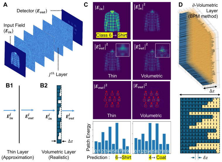
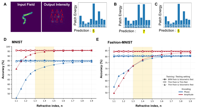
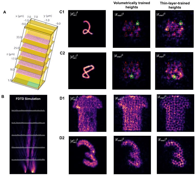
Replacing the thin-layer mask model with a differentiable beam-propagation layer that treats each neuron as a finite-thickness volume and propagates light through it during optimization produces fabrication-consistent visible-range diffractive networks whose full-wave FDTD performance reaches 90 percent accuracy on standard benchmarks.

What carries the argument

The differentiable beam-propagation (∂BPM) layer, which models each diffractive element as a finite-thickness volume and computes light propagation through it at training time.

If this is right

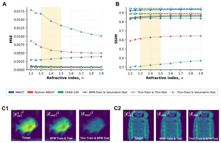
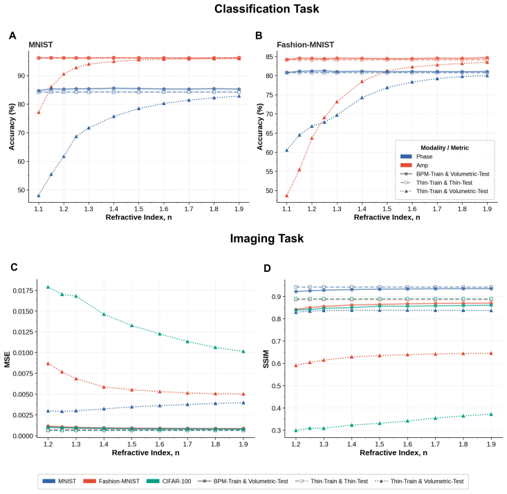
Design-to-device mismatch drops substantially across MNIST, Fashion-MNIST, and CIFAR-100 tasks.
Full-wave validation accuracy rises from 50 percent to 90 percent without re-optimization.
The same volumetric training applies to both classification and imaging objectives.
Height maps remain fabrication-compatible and end-to-end trainable without inserting full-wave solvers in the loop.

Where Pith is reading between the lines

These are editorial extensions of the paper, not claims the author makes directly.

The approach could be combined with actual nano-fabrication runs to test whether the simulated 90 percent accuracy survives real material and etch variations.
Similar volumetric modeling might be needed for other low-index platforms such as visible metasurfaces or integrated photonic circuits.
If the method generalizes, it would allow direct transfer of digitally optimized diffractive front-ends into compact visible cameras without digital post-processing.

Load-bearing premise

The beam-propagation method inside the differentiable layer accurately captures intra-layer diffraction and phase accumulation for the low-refractive-index relief structures used at visible wavelengths, without needing full-wave simulation during training.

What would settle it

A full-wave FDTD simulation or fabricated measurement of a ∂BPM-trained height map that still shows classification accuracy near 50 percent instead of 90 percent.

Figures

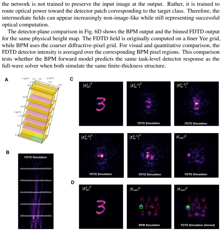
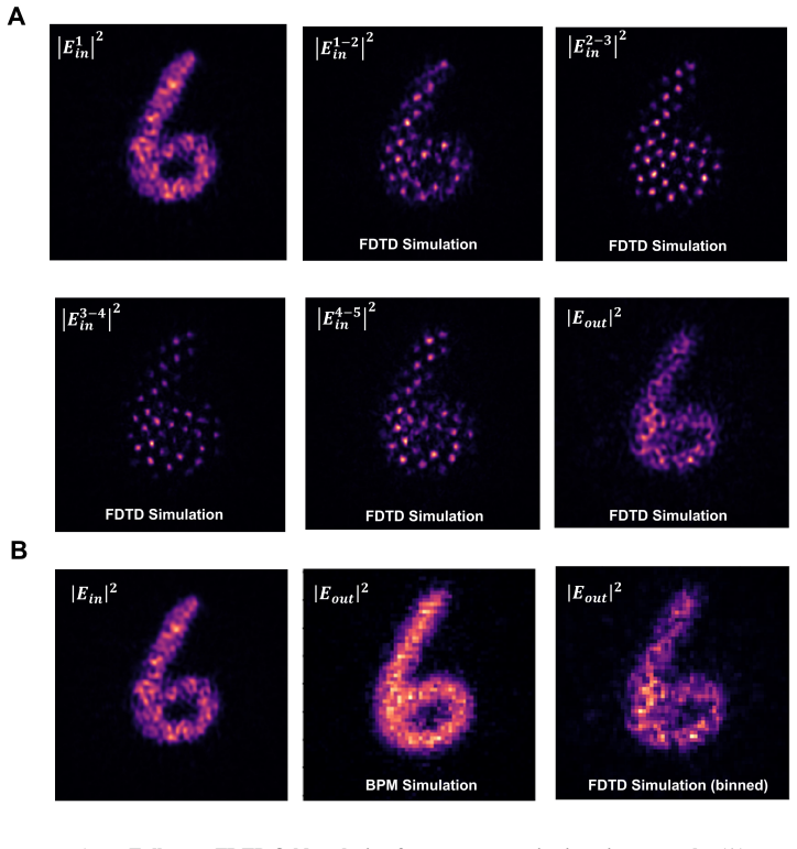
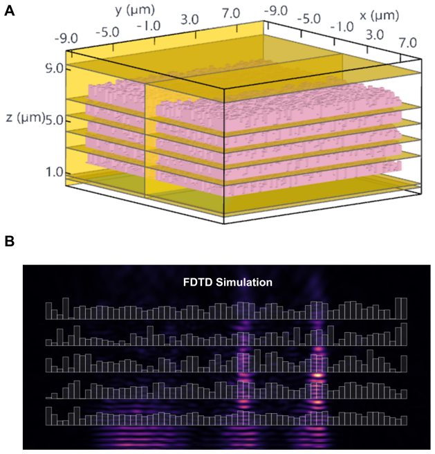
Figures reproduced from arXiv: 2606.07896 by Dineth Jayakody, Dushan N. Wadduwage.

**Figure 1.** Figure 1: The model mismatch issue due to the thin-layer approximation and the proposed differentiable volumetric layer based on BPM. (A) A schematic of a D2NN with an input field, five thin layers, and the field at the detector plane. (B1) A schematic of the thin-layer approximation used during training. (B2) A schematic of a realistic finite-thickness volumetric layer. (C) Representative fields at the input, immed… view at source ↗

**Figure 2.** Figure 2: Effect of model mismatch between thin-layer training and volumetric evaluation on optical classification. (A) Representative MNIST input, detector output, and patch-energy distribution for a thin-trained/thin-tested model. (B) The same thin-trained model evaluated with the finite-thickness volumetric forward model; the prediction becomes incorrect. (C) A BPM-trained model evaluated with the same volumetri… view at source ↗

**Figure 3.** Figure 3: Effect of model mismatch between thin-layer training and volumetric evaluation on optical imaging. (A) MSE for MNIST, Fashion-MNIST, and CIFAR100 imaging under thin-trained/thin-tested, thin-trained/volumetric-tested, and BPMtrained/volumetric-tested settings. (B) Corresponding SSIM values. The yellow shaded region highlights 𝑛 ≈ 1.3–1.5, a low/moderate-index range relevant to transparent visible-light-c… view at source ↗

**Figure 4.** Figure 4: Full-wave FDTD validation of volumetrically trained and thin-layertrained diffractive height maps. (A) Three-dimensional rendering of the five-layer finite-thickness diffractive structure used in FDTD simulation. (B) Cross-sectional FDTD field intensity along the propagation axis, showing intra-layer and inter-layer field evolution. (C1–C2) Classification examples evaluated directly in FDTD. The left colu… view at source ↗

**Figure 5.** Figure 5: Wavelength-scaled THz validation of the thin-to-volumetric model mismatch. The same normalized optical geometries used in the main experiments are instantiated at 𝜆 = 750 𝜇m, matching the THz wavelength used in the original free-space D2NN demonstration. (A–B) Classification accuracy for MNIST and Fashion-MNIST under phase and amplitude encoding. Thin-trained models degrade when evaluated with the volumetr… view at source ↗

**Figure 6.** Figure 6: Full-wave FDTD field evolution for a representative classification example. (A) Reconstructed finite-thickness diffractive stack used in the FDTD simulation. The learned height maps are implemented as volumetric dielectric structures rather than zero-thickness phase masks. (B) Longitudinal FDTD field slice through the diffractive stack, showing how the optical field evolves along the propagation direction … view at source ↗

**Figure 7.** Figure 7: Full-wave FDTD field evolution for a representative imaging example. (A) Transverse intensity monitors through the finite-thickness diffractive stack. Unlike the classification task, the imaging task aims to preserve the input spatial structure at the detector plane, so the output remains image-like after propagation through the diffractive layers. (B) Output comparison for the same sample. The target/inpu… view at source ↗

**Figure 8.** Figure 8: Finite-thickness FDTD geometry and longitudinal field propagation. (A) Three-dimensional view of the reconstructed diffractive stack used in the FDTD solver. The learned height maps are implemented as volumetric dielectric structures with nonzero axial thickness. (B) Longitudinal FDTD intensity slice through the structure. The field evolves continuously across the finite-thickness layers and freespace gap… view at source ↗

read the original abstract

Diffractive deep neural networks (D2NNs) promise miniaturized, power-efficient, light-speed optical front-ends for machine vision, yet the most mature demonstrations remain in the terahertz regime, built from readily fabricated millimeter-scale neurons. Translating D2NNs to the visible range, where nearly all vision pipelines operate, was long blamed on the difficulty of fabricating nanoscale neurons; but even after recent advances removed that barrier, visible-range D2NNs matching their terahertz counterparts remain out of reach. We identify the true obstacle as the thin-layer approximation underlying nearly all D2NN training, which treats each diffractive layer as an infinitely thin mask. It fails not because of the short wavelength, as is commonly assumed, but because the low-refractive-index materials (n approximately 1.3-1.5) used at visible wavelengths require relief structures thick enough that intra-layer diffraction and phase accumulation become significant. To overcome this, we introduce a differentiable beam-propagation ($\partial$BPM) layer that models each element as a finite-thickness volume and propagates light through it during training, keeping the fabrication-compatible height map end-to-end trainable without full-wave simulation in the loop. Across MNIST, Fashion-MNIST, and CIFAR-100 classification and imaging, $\partial$BPM training substantially reduces the design-to-device mismatch, and full-wave FDTD validation raises classification accuracy from 50% to 90% without re-optimization. The $\partial$BPM layer thus offers a scalable, physics-aware bridge between efficient optical neural-network optimization and fabrication-consistent diffractive design.

Editorial analysis

A structured set of objections, weighed in public.

Desk editor's note, referee report, simulated authors' rebuttal, and a circularity audit. Tearing a paper down is the easy half of reading it; the pith above is the substance, this is the friction.

Desk Editor's Note private letter to a colleague

The paper adds a differentiable volumetric BPM layer that improves FDTD-validated accuracy for visible D2NNs, but the validation details are too thin to confirm the physics is the real driver.

read the letter

The main takeaway is that they swap the usual thin-mask approximation for a differentiable beam-propagation layer that treats each diffractive element as a finite-thickness volume. This produces height maps that survive full-wave FDTD checks far better than thin-layer training, lifting accuracy from 50% to 90% on the reported tasks.

What is new is the ∂BPM operator itself. Prior D2NN work stays with infinitely thin phase masks; this one propagates light through the actual relief thickness during the forward and backward passes while keeping the fabrication-friendly height map trainable. That is a concrete technical step for visible wavelengths, where low-index materials force thicker structures and intra-layer effects matter.

The paper does a clear job naming the actual bottleneck. Fabrication advances have already made nanoscale neurons possible, yet performance stayed poor because the training model ignored thickness-dependent diffraction and phase. The volumetric approach directly targets that mismatch without forcing FDTD into every training step.

The soft spot is the validation. The abstract states the accuracy gain but supplies no dataset splits, error bars, run counts, or direct BPM-to-FDTD field comparison on the final devices. Without those numbers it is hard to tell whether the optimizer learned better physics or simply exploited BPM approximations that do not fully match the low-n, visible case.

The stress-test concern about paraxial limits, polarization, and evanescent effects is therefore still open. If the full paper includes quantitative field-error metrics between BPM and FDTD on the trained structures, that would close the gap; otherwise the central claim rests on an unexamined assumption.

This is for groups working on optical front-ends who need training methods that survive fabrication. It deserves peer review because the method is specific, the performance claim is testable, and the problem it addresses is real even if the current evidence needs tightening.

Referee Report

2 major / 2 minor

Summary. The paper claims that the thin-layer approximation fails for visible-range diffractive neural networks because low-index (n≈1.3-1.5) relief structures require thicknesses where intra-layer diffraction matters; it introduces a differentiable beam-propagation (∂BPM) layer that treats each diffractive element as a finite-thickness volume, enabling end-to-end training of fabrication-compatible height maps. Across MNIST, Fashion-MNIST and CIFAR-100 classification/imaging tasks, ∂BPM training reduces design-to-device mismatch, and post-training full-wave FDTD validation raises accuracy from ~50% to 90% without re-optimization.

Significance. If the central result holds, the work supplies a practical, scalable bridge between efficient gradient-based optimization of D2NNs and fabrication-consistent designs at visible wavelengths, where full-wave simulation in the training loop remains prohibitive. The explicit separation of the differentiable propagation operator from the FDTD validation step, together with the retention of a height-map parameterization, is a concrete strength that could be adopted by other groups working on volumetric diffractive optics.

major comments (2)

[Abstract / Results] Abstract and Results (performance claims): the reported FDTD-validated accuracy increase from 50% to 90% is presented without dataset splits, error bars, number of independent runs, or exclusion criteria; because this number is the primary quantitative support for the claim that ∂BPM reduces design-to-device mismatch, the absence of these controls is load-bearing for the central empirical result.
[Methods] Methods / ∂BPM layer definition: no quantitative BPM-versus-FDTD field-error metric (e.g., L2 field difference or phase RMSE) is supplied for the final trained structures; without this datum it remains possible that the optimizer exploits BPM-specific artifacts (paraxial or scalar approximations) rather than converging to a physically accurate solution, undermining the interpretation that the accuracy gain arises from correct intra-layer modeling.

minor comments (2)

[Methods] Notation: the symbol ∂BPM is introduced without an explicit statement of whether the split-step or angular-spectrum implementation is used and how polarization is (or is not) handled.
[Figures] Figure captions: several performance plots lack axis labels for the thin-layer baseline, making direct visual comparison with the ∂BPM curves difficult.

Simulated Author's Rebuttal

2 responses · 0 unresolved

We thank the referee for the constructive comments, which help strengthen the empirical foundation of the work. We address each major point below and will revise the manuscript to incorporate the requested details.

read point-by-point responses

Referee: [Abstract / Results] Abstract and Results (performance claims): the reported FDTD-validated accuracy increase from 50% to 90% is presented without dataset splits, error bars, number of independent runs, or exclusion criteria; because this number is the primary quantitative support for the claim that ∂BPM reduces design-to-device mismatch, the absence of these controls is load-bearing for the central empirical result.

Authors: We agree that the central performance claim requires more rigorous statistical reporting. In the revised manuscript we will explicitly state the dataset splits (standard 60 000/10 000 train/test for MNIST and Fashion-MNIST; 50 000/10 000/10 000 for CIFAR-100), report all accuracies as mean ± standard deviation over five independent training runs with distinct random seeds, and confirm that no data were excluded beyond the conventional splits. These details will appear in the Results section and, space permitting, the Abstract. revision: yes
Referee: [Methods] Methods / ∂BPM layer definition: no quantitative BPM-versus-FDTD field-error metric (e.g., L2 field difference or phase RMSE) is supplied for the final trained structures; without this datum it remains possible that the optimizer exploits BPM-specific artifacts (paraxial or scalar approximations) rather than converging to a physically accurate solution, undermining the interpretation that the accuracy gain arises from correct intra-layer modeling.

Authors: We acknowledge that a direct field-error metric would further rule out exploitation of BPM approximations. While the large FDTD-validated accuracy gain already indicates that the learned height maps are physically functional, we will add quantitative BPM-versus-FDTD comparisons (L2 field difference and phase RMSE) evaluated on the final trained structures in the revised Methods section. These metrics will be computed by propagating identical test fields through both the trained ∂BPM model and a full-wave FDTD solver. revision: yes

Circularity Check

0 steps flagged

No significant circularity; independent differentiable operator with external validation

full rationale

The paper defines a new differentiable beam-propagation (∂BPM) layer that models finite-thickness volumes, uses it for end-to-end training of height maps, and reports performance via external full-wave FDTD validation on standard datasets (MNIST, Fashion-MNIST, CIFAR-100). The accuracy gains (50% to 90%) are measured on held-out classification/imaging tasks and FDTD, not by construction from fitted parameters inside the same loop. No self-citation chains, self-definitional equations, fitted-input-as-prediction, or ansatz smuggling appear in the abstract or described chain; the method is self-contained against external benchmarks.

Axiom & Free-Parameter Ledger

0 free parameters · 1 axioms · 1 invented entities

The approach rests on the beam-propagation approximation being adequate for the target materials and thicknesses; no free parameters or invented entities are quantified in the abstract.

axioms (1)

domain assumption Beam propagation method sufficiently approximates intra-layer diffraction and phase accumulation for low-index relief structures at visible wavelengths
Invoked to justify replacing full-wave simulation inside the training loop.

invented entities (1)

∂BPM layer no independent evidence
purpose: Differentiable volumetric propagation operator inserted into the training pipeline
New component introduced to model finite thickness; no independent evidence supplied in abstract.

pith-pipeline@v0.9.1-grok · 5834 in / 1259 out tokens · 18430 ms · 2026-06-27T20:38:51.002786+00:00 · methodology

discussion (0)

Reference graph

Works this paper leans on

21 extracted references

[1]

All-optical machine learning using diffractive deep neural networks,

X. Lin, Y. Rivenson, N. T. Yardimci,et al., “All-optical machine learning using diffractive deep neural networks,” Science361, 1004–1008 (2018)

2018
[2]

Optical neural networks: progress and challenges,

T. Fu, J. Zhang, R. Sunet al., “Optical neural networks: progress and challenges,” Light. Sci. & Appl.13, 263 (2024)

2024
[3]

Diffractive deep neural networks: Theories, optimization, and applications,

H. Chen, S. Lou, Q. Wanget al., “Diffractive deep neural networks: Theories, optimization, and applications,” Appl. Phys. Rev.11, 021316 (2024)

2024
[4]

Diffractive optical computing in free space,

J. Hu, D. Mengu, D. C. Tzarouchis,et al., “Diffractive optical computing in free space,” Nat. Commun.15, 1525 (2024)

2024
[5]

Design of task-specific optical systems using broadband diffractive neural networks,

Y. Luo, D. Mengu, N. T. Yardimci,et al., “Design of task-specific optical systems using broadband diffractive neural networks,” Light. Sci. & Appl.8, 112 (2019)

2019
[6]

Terahertz pulse shaping using diffractive surfaces,

M. Veli, D. Mengu, N. T. Yardimci,et al., “Terahertz pulse shaping using diffractive surfaces,” Nat. Commun.12, 37 (2021)

2021
[7]

Learning diffractive optical communication around arbitrary opaque occlusions,

M. S. S. Rahman, T. Gan, E. A. Deger,et al., “Learning diffractive optical communication around arbitrary opaque occlusions,” Nat. Commun.14, 6830 (2023)

2023
[8]

Snapshot multispectral imaging using a diffractive optical network,

D. Mengu, A. Tabassum, M. Jarrahi, and A. Ozcan, “Snapshot multispectral imaging using a diffractive optical network,” Light. Sci. & Appl.12, 86 (2023)

2023
[9]

All-optical image denoising and feature enhancement using a diffractive visual processor,

c. Işı l, T. Gan, F. O. Ardicet al., “All-optical image denoising and feature enhancement using a diffractive visual processor,” Light. Sci. & Appl.13, 43 (2024)

2024
[10]

All-optical complex field imaging using diffractive processors,

J. Li, Y. Li, T. Gan,et al., “All-optical complex field imaging using diffractive processors,” Light. Sci. & Appl.13, 120 (2024)

2024
[11]

Pre-sensor computing with compact multilayer optical neural networks,

Z. Huanget al., “Pre-sensor computing with compact multilayer optical neural networks,” Sci. Adv.10, eado8516 (2024)

2024
[12]

Spectrally encoded single-pixel machine vision using diffractive networks,

J. Li, D. Mengu, N. T. Yardimci,et al., “Spectrally encoded single-pixel machine vision using diffractive networks,” Sci. Adv.7, eabd7690 (2021)

2021
[13]

All-optical phase conjugation using diffractive wavefront processing,

C.-Y. Shen, J. Liet al., “All-optical phase conjugation using diffractive wavefront processing,” Nat. Commun.15, 5406 (2024)

2024
[14]

Diffractive deep neural networks at visible wavelengths,

H. Chen, J. Feng, M. Jiang,et al., “Diffractive deep neural networks at visible wavelengths,” Engineering7, 1483–1491 (2021)

2021
[15]

Isotropic shrinkage of patterned vacancies enables three-dimensional nanoprecise metastructures for visible light applications,

Q. Yang, G. Yang, T. Nambara,et al., “Isotropic shrinkage of patterned vacancies enables three-dimensional nanoprecise metastructures for visible light applications,” Nat. Photonics pp. 1–11 (2026)

2026
[16]

Analysis of diffractive optical neural networks and their integration with electronic neural networks,

D. Mengu, Y. Luo, Y. Rivenson, and A. Ozcan, “Analysis of diffractive optical neural networks and their integration with electronic neural networks,” IEEE J. Sel. Top. Quantum Electron.26, 1–14 (2019)

2019
[17]

Tidy3d: Fastfdtdelectromagneticsolver,

FlexcomputeInc.,“Tidy3d: Fastfdtdelectromagneticsolver,”https://www.flexcompute.com/tidy3d/(2024).Accessed: 2026-03-20. Beyond the Thin-Layer Limit: Differentiable Volumetric Training for Visible-Range Diffractive Neural Networks - Supplementary Material

2024
[18]

Toverifythattheobservedthin-to-volumetricmismatchisnotspecifictothisabsolutewavelength, werepeatthesameBPMexperimentsunderawavelength-scaledTHzconfiguration

Validation at THz Wavelengths The main experiments in this work are reported at the visible wavelength of𝜆=532 nm , where low- and moderate-index transparent materials make finite-thickness effects especially relevant. Toverifythattheobservedthin-to-volumetricmismatchisnotspecifictothisabsolutewavelength, werepeatthesameBPMexperimentsunderawavelength-scal...
[19]

FDTD Simulation Details 2.1. FDTD source construction and numerical discretization For the BPM–FDTD validation experiments, the learned diffractive layers are exported as physical height maps and reconstructed as finite-thickness dielectric structures in the FDTD solver. The validation uses a matched64×64 diffractive-layer grid to keep the full-wave simul...
[20]

Consider an optical field𝑈(𝑥, 𝑦,0) at the input plane

Connection Between ASM Propagation, Evanescent Components, and the Neuron-Size Limit The angular spectrum method (ASM) provides a direct way to understand why the conventional diffraction-angle formula is no longer physically meaningful when the neuron size becomes smaller than𝜆/2. Consider an optical field𝑈(𝑥, 𝑦,0) at the input plane. In ASM, this field ...
[21]

We now connect this propagation limit to the geometric connectivity condition used for visible-wavelength𝐷2NN design

Derivation of the Inter-Layer Connectivity Condition The above neuron-size argument explains when a spatial-frequency component can propagate in free space. We now connect this propagation limit to the geometric connectivity condition used for visible-wavelength𝐷2NN design. In a free-space 𝐷2NN, the field diffracted by each neuron should spread sufficient...

[1] [1]

All-optical machine learning using diffractive deep neural networks,

X. Lin, Y. Rivenson, N. T. Yardimci,et al., “All-optical machine learning using diffractive deep neural networks,” Science361, 1004–1008 (2018)

2018

[2] [2]

Optical neural networks: progress and challenges,

T. Fu, J. Zhang, R. Sunet al., “Optical neural networks: progress and challenges,” Light. Sci. & Appl.13, 263 (2024)

2024

[3] [3]

Diffractive deep neural networks: Theories, optimization, and applications,

H. Chen, S. Lou, Q. Wanget al., “Diffractive deep neural networks: Theories, optimization, and applications,” Appl. Phys. Rev.11, 021316 (2024)

2024

[4] [4]

Diffractive optical computing in free space,

J. Hu, D. Mengu, D. C. Tzarouchis,et al., “Diffractive optical computing in free space,” Nat. Commun.15, 1525 (2024)

2024

[5] [5]

Design of task-specific optical systems using broadband diffractive neural networks,

Y. Luo, D. Mengu, N. T. Yardimci,et al., “Design of task-specific optical systems using broadband diffractive neural networks,” Light. Sci. & Appl.8, 112 (2019)

2019

[6] [6]

Terahertz pulse shaping using diffractive surfaces,

M. Veli, D. Mengu, N. T. Yardimci,et al., “Terahertz pulse shaping using diffractive surfaces,” Nat. Commun.12, 37 (2021)

2021

[7] [7]

Learning diffractive optical communication around arbitrary opaque occlusions,

M. S. S. Rahman, T. Gan, E. A. Deger,et al., “Learning diffractive optical communication around arbitrary opaque occlusions,” Nat. Commun.14, 6830 (2023)

2023

[8] [8]

Snapshot multispectral imaging using a diffractive optical network,

D. Mengu, A. Tabassum, M. Jarrahi, and A. Ozcan, “Snapshot multispectral imaging using a diffractive optical network,” Light. Sci. & Appl.12, 86 (2023)

2023

[9] [9]

All-optical image denoising and feature enhancement using a diffractive visual processor,

c. Işı l, T. Gan, F. O. Ardicet al., “All-optical image denoising and feature enhancement using a diffractive visual processor,” Light. Sci. & Appl.13, 43 (2024)

2024

[10] [10]

All-optical complex field imaging using diffractive processors,

J. Li, Y. Li, T. Gan,et al., “All-optical complex field imaging using diffractive processors,” Light. Sci. & Appl.13, 120 (2024)

2024

[11] [11]

Pre-sensor computing with compact multilayer optical neural networks,

Z. Huanget al., “Pre-sensor computing with compact multilayer optical neural networks,” Sci. Adv.10, eado8516 (2024)

2024

[12] [12]

Spectrally encoded single-pixel machine vision using diffractive networks,

J. Li, D. Mengu, N. T. Yardimci,et al., “Spectrally encoded single-pixel machine vision using diffractive networks,” Sci. Adv.7, eabd7690 (2021)

2021

[13] [13]

All-optical phase conjugation using diffractive wavefront processing,

C.-Y. Shen, J. Liet al., “All-optical phase conjugation using diffractive wavefront processing,” Nat. Commun.15, 5406 (2024)

2024

[14] [14]

Diffractive deep neural networks at visible wavelengths,

H. Chen, J. Feng, M. Jiang,et al., “Diffractive deep neural networks at visible wavelengths,” Engineering7, 1483–1491 (2021)

2021

[15] [15]

Isotropic shrinkage of patterned vacancies enables three-dimensional nanoprecise metastructures for visible light applications,

Q. Yang, G. Yang, T. Nambara,et al., “Isotropic shrinkage of patterned vacancies enables three-dimensional nanoprecise metastructures for visible light applications,” Nat. Photonics pp. 1–11 (2026)

2026

[16] [16]

Analysis of diffractive optical neural networks and their integration with electronic neural networks,

D. Mengu, Y. Luo, Y. Rivenson, and A. Ozcan, “Analysis of diffractive optical neural networks and their integration with electronic neural networks,” IEEE J. Sel. Top. Quantum Electron.26, 1–14 (2019)

2019

[17] [17]

Tidy3d: Fastfdtdelectromagneticsolver,

FlexcomputeInc.,“Tidy3d: Fastfdtdelectromagneticsolver,”https://www.flexcompute.com/tidy3d/(2024).Accessed: 2026-03-20. Beyond the Thin-Layer Limit: Differentiable Volumetric Training for Visible-Range Diffractive Neural Networks - Supplementary Material

2024

[18] [18]

Toverifythattheobservedthin-to-volumetricmismatchisnotspecifictothisabsolutewavelength, werepeatthesameBPMexperimentsunderawavelength-scaledTHzconfiguration

Validation at THz Wavelengths The main experiments in this work are reported at the visible wavelength of𝜆=532 nm , where low- and moderate-index transparent materials make finite-thickness effects especially relevant. Toverifythattheobservedthin-to-volumetricmismatchisnotspecifictothisabsolutewavelength, werepeatthesameBPMexperimentsunderawavelength-scal...

[19] [19]

FDTD Simulation Details 2.1. FDTD source construction and numerical discretization For the BPM–FDTD validation experiments, the learned diffractive layers are exported as physical height maps and reconstructed as finite-thickness dielectric structures in the FDTD solver. The validation uses a matched64×64 diffractive-layer grid to keep the full-wave simul...

[20] [20]

Consider an optical field𝑈(𝑥, 𝑦,0) at the input plane

Connection Between ASM Propagation, Evanescent Components, and the Neuron-Size Limit The angular spectrum method (ASM) provides a direct way to understand why the conventional diffraction-angle formula is no longer physically meaningful when the neuron size becomes smaller than𝜆/2. Consider an optical field𝑈(𝑥, 𝑦,0) at the input plane. In ASM, this field ...

[21] [21]

We now connect this propagation limit to the geometric connectivity condition used for visible-wavelength𝐷2NN design

Derivation of the Inter-Layer Connectivity Condition The above neuron-size argument explains when a spatial-frequency component can propagate in free space. We now connect this propagation limit to the geometric connectivity condition used for visible-wavelength𝐷2NN design. In a free-space 𝐷2NN, the field diffracted by each neuron should spread sufficient...