REVIEW 4 major objections 5 minor 10 references
Machine-Precision Prediction of Low-Dimensional Chaotic Systems from Noise-Free Data
T0 review · 4 major / 5 minor · reviewed 2026-08-06 · deepseek-v4-flash
Pith's one-line read Noise-free forecasting of low-dimensional chaos is effectively solved: polynomial regression in 512-bit arithmetic matches or beats 64-bit solvers that know the true equations, reaching 105 Lyapunov times on Lorenz-63.
desk verdict Record VPTs from a high-precision polynomial propagator, but the benchmark is relative to a fixed RK4 integrator and the best numbers are selected on the test set; still deserves a serious referee. read the letter →
The pith
A machine-rendered reading of the paper's core claim, the machinery that carries it, and where it could break.
The reading
What carries the argument
The load-bearing object is the polynomial propagator: the map $\hat\Phi_{\Delta t}(s) = \hat\beta^\top \xi_p(s)$ obtained by ordinary least squares, where $\xi_p$ stacks all monomials of degree $\le p$ in the $d$ state coordinates and $\hat\beta = (X^\top X)^{-1}X^\top Y$ solves the normal equations. Its two supporting mechanisms are high-precision linear algebra (512-bit arithmetic) to handle the ill-conditioned design matrix, and an auxiliary structural fact: the exact propagator of the RK4 integrator applied $k$ times to the Lorenz-63 equations is a polynomial of degree $F_{4k+2}$, the $(4k+2)$-nd Fibonacci number, so a single RK4 step is exactly a degree-$8$ polynomial. That identity explains why moderate-degree fits saturate the solver's own accuracy when the data step equals the solver step, and why sub-sampling the solver output (two steps already give degree 55) makes the learning task intrinsically harder.
What would settle it
Generate training and test data from a qualitatively different high-accuracy reference, for example an adaptive-step solver or a Taylor-method integrator with error control, and rerun the default configuration: if the 32 to 105 Lyapunov-time valid predictions persist, they reflect the underlying dynamics, while a collapse toward the 13 Lyapunov-time regime would show the result is specific to imitating the RK4 map. A second, cheaper check is to inject deterministic rounding noise into the last stored bit of the 64-bit training data and measure the valid prediction time as a function of that noise level.
Extended reading notes
Core claim
The paper's central claim is that a system-agnostic forecaster, namely ordinary least squares regression of the propagator $u(t)\mapsto u(t+\Delta t)$ on the multivariate monomials of the current state, reaches the numerical accuracy of the RK4 integrator that generated the data, and in the best configurations slightly exceeds it. The achievement is not a clever statistical model but numerical hygiene: high-degree polynomial features make the normal equations extremely ill-conditioned, and the paper shows that 512-bit arithmetic with full data normalization removes that bottleneck, while a 32-bit or 64-bit pipeline caps out near 7 or 21 Lyapunov times. Because the training data is noise-free, regularization is counterproductive and OLS is the right estimator. In the default setup (512-bit solver, 64-bit stored data, 512-bit fitter) the learned propagator reaches a valid prediction time of 35.6 Lyapunov times on Lorenz-63 versus 32.1 for a 64-bit RK4 solver, and with 512 bits used end to end it reaches 105 Lyapunov times, a ceiling the authors attribute to their chosen degree bound rather than to the method.
Load-bearing premise
The whole comparison treats the output of one particular numerical solver, run at one fixed time step, as the true system: the polynomial learns to imitate that solver's discrete map rather than the exact continuous-time equations, so the claimed machine-precision ceiling is relative to that solver.
Editorial extensions
If this is right
- On Lorenz-63, previously published methods top out near 13 Lyapunov times; this method reaches 32 to 36 in realistic precision configurations and 105 when data and computation are both carried at 512-bit precision, averaged over 100 initial conditions.
- The learned propagator outperforms a 64-bit RK4 solver of the true equations in the default setup (35.6 versus 32.1 Lyapunov times), so a data-only forecast can be more accurate than a standard solver that is handed the exact vector field.
- The results transfer to the non-polynomial Thomas' Cyclically Symmetric Attractor, where degree-25 polynomials match a 512-bit solver at 38.0 Lyapunov times, showing the success does not depend on the vector field being polynomial.
- For the spatiotemporally chaotic Lorenz-96 model in dimensions 5 through 9, the method reaches single-precision machine accuracy, with valid prediction times statistically indistinguishable from the reference solver's.
- Forecasting from a single state (random test mode) performs as well as continuing from the training trajectory, because the estimated propagator depends only on the current state.
- The authors draw the practical conclusion that noise-free Lorenz-63-style benchmarks are too easy to discriminate among methods, and that future work on learning dynamical systems should focus on noisy data.
Reading between the lines
- If the claim holds, the relevant question shifts from 'can we learn the system' to 'where does the precision floor sit': the error budget is set by the least precise component of the data pipeline, so adding deterministic rounding noise at the level of the last stored bit should visibly cut the achievable valid prediction time, a cheap testable extension of the paper's own logic.
- Because the fitted object is the discrete integrator map, the method's machine-precision result is relative to whatever solver generated the data; training on RK4 output and validating against a radically different high-accuracy integrator would separate 'learning the continuous dynamics' from 'imitating the solver', which the paper does not test.
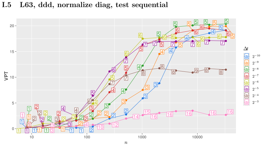
- The observed preference for a medium data step ($\Delta t \approx 2^{-5}$) over finer sampling suggests a trade-off between propagator simplicity and state-space exploration; sweeping $n$ beyond $2^{15}$ and degree beyond 16 could map where the 105-Lyapunov-time ceiling actually moves.
- The authors' own caveat that dimensions of order 100 are computationally infeasible implies the method's success is tied to low dimension; applying it to moderately high-dimensional or noisy settings is where the 'solved problem' conclusion is most likely to break.
Editorial analysis
A structured set of objections, weighed in public.
Referee Report
Summary. The paper proposes a system-agnostic forecasting method that fits high-degree polynomial features to the discrete-time propagator of a chaotic system using ordinary least squares, executed in 512-bit arithmetic. On Lorenz-63, it reports valid prediction times of about 35.6 Lyapunov times in the default setup and up to 104.9 (or 322 at the solver step size) with 512-bit data, far exceeding prior ML results and slightly exceeding the 64-bit RK4 solver baseline. The method is also applied to Thomas' Cyclically Symmetric Attractor and Lorenz-96 in dimensions 5 through 9, where it matches the respective solver baselines. All training and test trajectories are generated by the authors' fixed RK4 integrator, and the VPT is evaluated against that same discrete reference.
Significance. If the claims are read as "the method reproduces the data-generating discrete map at machine precision," the results are substantial: the empirical design is thorough, with 100 repetitions per configuration, confidence intervals, a Zenodo data release, and a formal proof in Appendix G that k RK4 steps of L63 are a polynomial of Fibonacci degree. The method is simple, data-efficient, and makes falsifiable predictions that prior ML benchmarks consistently fail to reach. However, the current abstract and title claim accuracy relative to "the true underlying dynamical systems," which is not established because the ground truth is always the output of one fixed RK4 integrator. This overstatement materially tempers the significance and needs to be addressed.
major comments (4)
- [Abstract; §1; §2.4; §3.1] The load-bearing claim that the method "exceeds the accuracy of standard 64-bit numerical ODE solvers of the true underlying dynamical systems" is not supported by the experiments, because the ground truth is always the output of the authors' fixed RK4 integrator with dt0=2^-10 (L63/L96) or 2^-6 (TCSA), and the same solver output is used for training and for VPT evaluation (Section 2.4, Table 6). The polynomial propagator therefore fits the discrete RK4 map, not the continuous-time flow; Appendix G makes this explicit by proving that one RK4 step of L63 is exactly a degree-8 polynomial, and Section 3.2 reports more than 322 Lyapunov times in the dt=dt0 case "because one RK4 solver step of the L63 system amounts to a polynomial propagator of degree 8." I recommend either reframing the abstract and title claims as matching or exceeding 64-bit solvers on the same discrete data-generating map, or adding an experiment that trains on the RK4 data and evaluates against a different high-accuracy reference (e.g., a much smaller-step 512-bit integration or a different integration scheme) to show that the learned propagator tracks the continuous flow itself.
- [§3.4; Table 3] The Lorenz-96 claims of "single-precision machine accuracy" and of results "statistically indistinguishable" from the solver share the same discrete-map limitation: both the training data and the RK4 reference forecast are generated by the same RK4 solver at the same dt0, so the comparison quantifies how well the polynomial propagator emulates the RK4 map given single-precision initial data, not how well it approximates the continuous-time Lorenz-96 flow. The equivalence test is also informal: "statistically indistinguishable" is defined as the solver's VPT lying inside the 95% confidence interval of the method, which with 100 repetitions and interval widths around ±0.8 Lyapunov times provides only weak evidence of equivalence; a formal test or a stated equivalence margin would be more appropriate.
- [§4 (Discussion); §3.2 (Figure 7)] The sentence "chaotic systems can be predicted to arbitrary accuracy—and thus arbitrary valid times" overreaches the evidence. All reported VPT values are for a fixed polynomial degree bound (p <= 16, or 25 for TCSA) and for a fixed data precision; the paper's own analysis (Figure 5 and Appendix C) shows the forecast error floor is set by the 64-bit data rounding, and no convergence result in p and n is proved. The claim should be narrowed to "arbitrary accuracy in reproducing the discrete-time propagator, up to the precision of the stored data and within the chosen polynomial feature family."
- [§3.2; Appendix G] The statement that the dt=dt0 result "is not a concern for larger time steps" is insufficient, because every VPT value in Table 2, including the headline 35.6 and 104.9 values, is measured against the same RK4-generated reference trajectory. The distinction between (a) exactly recovering the RK4 map when dt=dt0 and (b) approximating the map of the continuous-time system needs to be drawn in the methods and reflected in the interpretation of the headline results; otherwise readers will take "machine precision" to refer to the ODE flow rather than to the fixed numerical scheme.
minor comments (5)
- [Appendix A] The heading "Layapunov Exponent" is a typo and should read "Lyapunov Exponent."
- [Table 1; Figure 1; Appendix I captions] Several captions and labels contain stray spaces such as "V alid", "T raining", "T est", and "T ruth"; these should be cleaned up.
- [§2.4, Eq. (13)] The diagonal normalization is written with \hat{\sigma}^2_i inside a diagonal matrix, but the notation is ambiguous; please define \hat{S} explicitly as diag(\hat{\sigma}^2_1, ..., \hat{\sigma}^2_d) and clarify how \hat{S}^{-1/2} is computed.
- [§3.1, Figure 5] The plateau of constant error for about 8 Lyapunov times is an artifact of comparing a 512-bit forecast against 64-bit stored ground truth; the text should state this explicitly so readers do not attribute the plateau to the physics of the Lorenz system.
- [§4.2] The statement "there is no noise to overfit to" is too categorical, since finite-sample variance and multicollinearity of high-degree monomial bases are present even for noise-free data; the poor performance at small n and high degree visible in the Appendix I tables suggests these effects matter and deserve a sentence of qualification.
Circularity Check
No significant circularity: VPT is measured on held-out continuations; the one self-citation is peripheral and not load-bearing.
full rationale
The paper's central derivation is self-contained. A polynomial propagator is estimated by OLS regression on noise-free observations (Section 2.3, Eq. 9) and then iterated from a starting state; the reported VPT is evaluated against a held-out continuation or, in random test mode, against a new trajectory from a randomly chosen attractor state (Appendix E). The target is not used in fitting, and VPT is not a fitted parameter. The extreme value of more than 322 Lyapunov times at dt = dt0 is explicitly explained in Section 3.2 and Appendix G as a consequence of the RK4 one-step map of L63 being exactly a degree-8 polynomial; the model class therefore contains the target, which explains the result but is not circular because the polynomial coefficients are obtained by regression rather than by construction. The comparison with 64-bit RK4 solvers uses independently integrated trajectories from the same step size and different arithmetic precision (Table 6), which is a legitimate empirical benchmark. The only self-citation that could be questioned, the claim about poor performance under noise attributed to Schotz et al. [Sch+25] in Section 4.2, is peripheral to the central claim and not load-bearing. The main caveat, that ground truth is the output of a fixed RK4 integrator rather than the exact continuous-time flow, is a validity limitation of the benchmark rather than a circularity of the derivation.
Assumptions & free parameters
free parameters (3)
- polynomial degree p =
1 to 16 for L63/L96, up to 25 for TCSA
- data time step Delta t =
2^-10 to 2^-3 for L63, 2^-9 to 2^-5 for L96, 2^-6 to 2^1 for TCSA
- data normalization scheme =
none, diagonal, or full
assumptions (5)
- domain assumption The numerical output of the RK4 solver with fixed time step Delta t0 is accepted as ground truth for the true dynamical system.
- domain assumption The training trajectory explores the attractor well enough for the OLS-fitted polynomial propagator to generalize to unseen test states.
- domain assumption The linear system X^T X can be solved accurately at the chosen arithmetic precision.
- domain assumption The propagator of the system is sufficiently smooth over the attractor to be approximated by a degree-p polynomial to the needed accuracy.
- standard math Standard existence and uniqueness of ODE solutions holds for the studied systems.
Cite this review
Pith. "Pith review of Machine-Precision Prediction of Low-Dimensional Chaotic Systems from Noise-Free Data." pith.science (2026). https://pith.science/paper/GAXT4SWN
@misc{pith2026250709652,
  author       = {Pith},
  title        = {Pith review of: Machine-Precision Prediction of Low-Dimensional Chaotic Systems from Noise-Free Data},
  year         = {2026},
  howpublished = {\url{https://pith.science/paper/GAXT4SWN}},
  note         = {Machine review of arXiv:2507.09652}
}
read the original abstract
Low-dimensional chaotic systems such as the Lorenz-63 model are commonly used to benchmark system-agnostic methods for learning dynamics from data. This study shows that learning from noise-free observations in such systems can be achieved up to machine precision: using ordinary least squares regression on high-degree polynomial features with 512-bit arithmetic, a system-agnostic method is introduced that matches the accuracy of standard 64-bit numerical ODE solvers using the systems' governing equations. For the Lorenz-63 system, the method achieves valid prediction times of 36 Lyapunov times, and even up to 105 Lyapunov times with favorable precision configurations, dramatically outperforming prior work, which reaches 13 Lyapunov times at most. The results are further validated on Thomas' Cyclically Symmetric Attractor, a non-polynomial chaotic system that is considerably more complex than the Lorenz-63 model, and similar results extend to higher dimensions using the spatiotemporally chaotic Lorenz-96 model. These findings suggest that forecasting low-dimensional chaotic systems from noise-free data is effectively a solved problem.
Figures


Figures from the paper (69 more)




Reference graph
Works this paper leans on
-
[1]
[AT22] T. Akiyama and G. Tanaka. “Computational Efficiency of Multi-Step Learning Echo State Networks for Nonlinear Time Series Prediction”. In: IEEE Access 10 (2022), pp. 28535–28544. doi: 10.1109/access.2022.3158755. [Ben+80a] G. Benettin, L. Galgani, A. Giorgilli, and J.-M. Strelcyn. “Lyapunov Characteristic Exponents for smooth dynamical systems and f...
arXiv 2022
-
[7]
PySINDy: A Python package for the sparse identification of nonlinear dynamical systems from data
doi: 10 . 48550 / arXiv . 2407 . 20158. arXiv: 2407 . 20158 [cs.LG]. [Sil+20] B. M. de Silva, K. Champion, M. Quade, J.-C. Loiseau, J. N. Kutz, and S. L. Brunton. “PySINDy: A Python package for the sparse identification of nonlinear dynamical systems from data”. In: Journal of Open Source Software 5.49 (2020), p
work page 2020
-
[9]
Deterministic chaos seen in terms of feedback circuits: analysis, synthesis, “Labyrinth chaos
doi: 10.1201/9780429398490. [Tho99] R. Thomas. “Deterministic chaos seen in terms of feedback circuits: analysis, synthesis, “Labyrinth chaos””. In: International Journal of Bifurcation and Chaos 09.10 (1999), pp. 1889–1905. doi: 10.1142/S0218127499001383. [Vis04] D. Viswanath. “The fractal property of the Lorenz attractor”. In: Phys. D 190.1-2 (2004), pp...
-
[13]
Chaotic attractor reconstruction using small reservoirs—the influence of topology
[Jau24] L. Jaurigue. “Chaotic attractor reconstruction using small reservoirs—the influence of topology”. In: Machine Learning: Science and Technology 5.3 (Aug. 2024), p. 035058. doi: 10.1088/2632-2153/ad6ee8. [K¨ os+23] F. K¨ oster, D. Patel, A. Wikner, L. Jaurigue, and K. L¨ udge. “Data-informed reservoir computing for efficient time-series prediction”....
-
[2019]
Long-term Forecasting using Higher Order Tensor RNNs
doi: 10.48550/arXiv.1711.00073 . arXiv: 1711.00073 [cs.LG]. 91
-
[2020]
Neural Networks for Lorenz Map Prediction: A Trip Through Time
doi: 10.48550/arXiv.1903.07768. arXiv: 1903.07768 [cs.LG]. [SC25] C. Sanderson and R. Curtin. “Armadillo: an Efficient Framework for Numerical Linear Algebra”. In: 2025 17th International Conference on Computer and Automation En- gineering (ICCAE). 2025, pp. 303–307. doi: 10.1109/ICCAE64891.2025.10980539. 90 [Sch+25] C. Sch¨ otz, A. White, M. Gelbrecht, a...
work page Pith review arXiv doi:10.48550/arxiv.1903.07768 1903
-
[2022]
Using machine learning to replicate chaotic attractors and calculate Lyapunov exponents from data
doi: https://doi.org/ 10.48550/arXiv.2109.13406. arXiv: 2109.13406 [cs.MS]. [Ott02] E. Ott. Chaos in dynamical systems. Second. Cambridge University Press, Cambridge, 2002, pp. xii+478. doi: 10.1017/CBO9780511803260. MR 1924000. [Pat+17] J. Pathak, Z. Lu, B. R. Hunt, M. Girvan, and E. Ott. “Using machine learning to replicate chaotic attractors and calcul...
-
[2024]
Theoretical basis and application of an analogue-dynamical model in the Lorenz system
[Ren+09] H. Ren, J. Chou, J. Huang, and P. Zhang. “Theoretical basis and application of an analogue-dynamical model in the Lorenz system”. en. In: Adv. Atmos. Sci. 26.1 (Jan. 2009), pp. 67–77. [Rob20] D. Roberts. Neural Networks for Lorenz Map Prediction: A Trip Through Time
work page 2009
Show all 10 references
- [2025]
-
[2104]
Predicting three-dimensional chaotic systems with four qubit quantum systems
doi: 10.21105/joss.02104. [SR25] J. Steinegger and C. R¨ ath. “Predicting three-dimensional chaotic systems with four qubit quantum systems”. In: Scientific Reports 15.1 (Feb. 2025). doi: 10 . 1038 / s41598-025-87768-0 . [Sti74] S. M. Stigler. “Gergonne’s 1815 paper on the des...
1974 doi
Reviewed August 6, 2026 · model on record in the stance chip above.
Discussion (0). Continue with ORCID to comment.