REVIEW 2 major objections 5 minor 34 references
Score Matching With Missing Data
T0 review · 2 major / 5 minor · reviewed 2026-08-07 · deepseek-v4-flash
Pith's one-line read This paper adapts score matching to training data with coordinates missing completely at random, proving that minimising a marginal score-matching objective recovers the true full-data score, and giving two practical algorithms.
desk verdict Solid IW-based score matching for MCAR data, but the variational proof has a genuine θ-gradient error and the 'any score model' claim is overstated. read the letter →
The pith
A machine-rendered reading of the paper's core claim, the machinery that carries it, and where it could break.
The reading
What carries the argument
The central object is the marginal score function $s_\lambda(x_\lambda) = \nabla_{x_\lambda}\log \int q(x)\,dx_{-\lambda}$ for an unnormalised density $q$, with $s_{\lambda;\theta}$ defined analogously. Proposition 4.3 shows the marginal Fisher divergence $F_M(\theta)=E[\|s_\Lambda(X_\Lambda)-s_{\Lambda;\theta}(X_\Lambda)\|^2]$ equals the computable objective $L_M(\theta)$ plus a constant. The importance-weighting estimator replaces the intractable marginal score integral by a self-normalised Monte Carlo ratio. Lemma 4.8 supplies the gradient-first identities $s_{\theta;\lambda}(x_\lambda)=E'[s_\theta(x_\lambda,X'_{-\lambda})_\lambda]$ and $\nabla E'[h_\theta]=E'[\nabla h_\theta]+\mathrm{Cov}'(s_\theta,h_\theta)$, which turn the objective into expectations and covariances under the model's conditional $p_\theta(\cdot|x_\lambda)$ and permit black-box variational approximation.
What would settle it
Take two different two-dimensional densities with identical one-dimensional marginals, for example a Gaussian and a mixture with the same marginals but different dependence. If missingness only ever leaves one coordinate observed, the marginal objective cannot distinguish them; checking whether the minimiser is the true joint density would directly test Proposition 4.3, and the recovery should fail whenever the identifiability assumption is violated.
Extended reading notes
Core claim
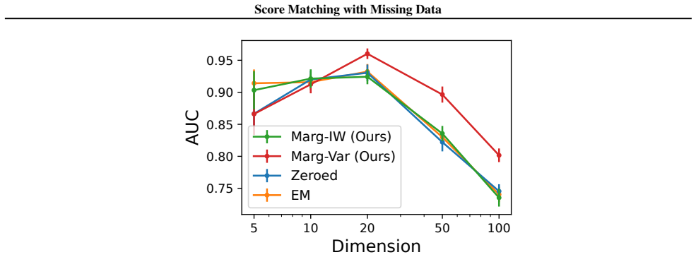
The paper claims that for missing-completely-at-random data, the marginal Fisher divergence between the model's marginal score and the true marginal score is equivalent—up to a constant—to an expectation that depends only on the model, so it can be minimised from partial observations. Under an identifiability assumption, any minimiser of this marginal objective is the true unnormalised density almost surely. For truncated domains, the importance-weighted version of the objective has a high-probability finite-sample bound: the marginal truncated Fisher divergence of the estimated score decays at roughly $\sqrt{\log(dnrA/\delta)/\min\{r,n\}}$. The variational variant re-expresses the gradient of the objective in terms of conditional expectations and covariances under the model, which can be approximated by a learned conditional distribution, and is the variant that performs best in high-dimensional graphical model experiments.
Load-bearing premise
The whole construction assumes your score model is the gradient of a known unnormalised density $q_\theta$, so the marginal score can be written as an integral of that density; if you only have a black-box score network with no anti-derivative, neither algorithm can be run.
Editorial extensions
If this is right
- Explicit parametric score models—Gaussian scores, energy-based models, and graphical-model precisions—can be trained on missing-completely-at-random data without imputation, by plugging $q_\theta$ into either algorithm.
- With the importance-weighting method on bounded domains, choosing $r$ proportional to $n$ importance samples per observation gives roughly $1/\sqrt{n}$ error in the marginal truncated Fisher divergence, at an $O(n^2)$ computational cost.
- Both algorithms extend to truncated, sliced, and denoising score matching, so the same marginalisation machinery can reach diffusion-style objectives.
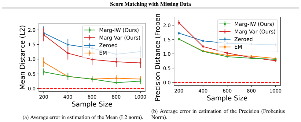
- In the paper's experiments, the variational variant recovers Gaussian graphical model edges from missing data with higher AUC than zero-imputation baselines, especially for structured graphs and higher dimensions.
Reading between the lines
- If the missingness patterns only expose marginals that do not pin down the joint distribution, the identifiability assumption fails; a practical diagnostic would be to check whether the observed-coordinate marginals determine the model family before trusting the recovered full-data score.
- The finite-sample guarantee is for the marginal objective, not the full-data score; a natural testable extension is to measure full-score error directly and see whether the same convergence rate survives.
- The requirement of a known unnormalised density $q_\theta$ suggests a next step: parameterising neural scores as gradients of a potential network, or learning a separate potential, would let the same objectives apply to general black-box score models.
Editorial analysis
A structured set of objections, weighed in public.
Referee Report
Summary. The paper extends score matching to missing data under the missing-completely-at-random assumption. It defines marginal scores and shows in Proposition 4.3 that the marginal Fisher divergence can be optimized through an integration-by-parts objective that involves only the marginal score model and its divergence. Since marginal scores are intractable, the authors propose an importance-weighting estimator of the marginal score (Section 4.2, Algorithm 1) and a variational estimator that approximates the conditional expectations and covariances in the parameter gradient (Section 4.3, Algorithm 2, Corollary 4.9). The paper further derives finite-sample high-probability bounds for truncated importance-weighted score matching (Theorem 4.6 and Appendix A.15), extends the framework to sliced, denoised, and missing-not-at-random settings, and reports experiments on truncated Gaussian, non-Gaussian, Gaussian graphical model, S&P 100, and yeast data.
Significance. The population-level equivalence in Proposition 4.3 is a clean and useful extension of the classical score-matching identity to marginal observations, and the finite-sample bound in Theorem 4.6/Appendix A.15 is more detailed than is typical for such estimators. The paper ships code and is candid about an important limitation: the bounds are for the marginal Fisher divergence, not for the full-data score error (Remark 4.7 and Section 6). However, the advertised scope of any parameterised score model exceeds what the algorithms actually require, and the variational method rests on Lemma 4.8, which is false as stated for θ-gradients. Both issues are fixable, but they need to be addressed before the claims can be accepted.
major comments (2)
- [Lemma 4.8; Appendix C.3; Corollary 4.9; Lemma A.18] The identity in Lemma 4.8, Eq. (9), is stated for ∇ equal to either ∇_{x_λ} or ∇_θ, but it is false for ∇ = ∇_θ. For ∇ = ∇_θ, the log-derivative computation gives ∇_θ E'[h_θ] = E'[∇_θ h_θ] + Cov'(∇_θ log q_θ, h_θ), not Cov'(s_θ, h_θ) with s_θ = ∇_x log q_θ. In the proof in Appendix C.3, the step replacing s_{θ;λ}(x_λ) E'[g_θ] by E'[∇ log p_θ(x_λ, X'_−λ)] E'[g_θ] is valid only when ∇ is the x_λ-gradient; for ∇ = ∇_θ the correct factor is E'[∇_θ log p_θ] E'[g_θ]. The same conflation appears in Lemma A.18. Because Corollary 4.9 and Algorithm 2 invoke Eq. (9), the derivation of the variational method is formally invalid as written; the displayed Ψ_Λ in Eq. (10) uses the correct ∇_θ log q_θ covariance, so the formula may be salvageable, but the lemma and its proof must be corrected before the claim can be accepted.
- [§1 vs. §4.1, Algorithms 1–2] The introduction claims compatibility with any parameterised score model and names neural networks as an example, but this is not supported by the algorithms. Definition 4.4 and Eq. (7) evaluate q_θ directly, Algorithm 1 takes q_θ as input, and the variational Ψ_Λ in Corollaries 4.9 and 4.11 requires ∇_θ log q_θ. A general neural-network score s_θ without a known anti-derivative cannot be used, and no construction is supplied. The actual scope is explicit unnormalised-density/energy models of the form s_θ = ∇_x log q_θ; the abstract, introduction, and the final remark in Section 5 that the methods can be applied to NNs should be revised to state this restriction.
minor comments (5)
- [Assumption 4.2] The assumption is introduced as 'For any θ > 0', but θ is a parameter vector; it should read 'For any θ ∈ Θ'.
- [Theorem 4.6 and Theorem A.15] The main-text bound is a substantial simplification of Appendix Theorem A.15; the constants β_i and the additional β_3((n+r)/(nr))(...) term are not defined in Section 4.2.2. Please state that the displayed rate is a simplified corollary of A.15 and point explicitly to the full statement.
- [Figure 2] The caption says 'Average Fisher Divergence for Gaussian score estimates', but the experiment in Section 5.1.2 measures θ-error for the non-Gaussian ICA-style model; the caption should say 'Theta Error'.
- [Assumption A.13] In the displayed inequality, the right-hand side should compare f_{l,λ}(x,θ) with f_{l,λ}(x,θ'), not with f_{0,λ}(x,θ'); as written the Lipschitz condition is mis-stated.
- [Appendix C.2, Proposition C.5] The proof contains a set-inclusion in the wrong direction: it writes {|Z_r(θ)-Z(θ)|<ε} ⊆ ∪_k E_k(θ), but the argument needs the complementary inclusion for the large-deviation event; please correct this typo so the union bound is applied to {|Z_r(θ)-Z(θ)|>ε}.
Circularity Check
No circularity: the marginal and truncated objectives are derived in-paper from standard score-matching integration-by-parts identities, and the sole overlapping-author citation (Liu et al. 2022) is an independently published theorem that is also re-derived in Appendix C.1.1.
full rationale
The paper's derivation chain is self-contained rather than circular. Proposition 4.3 obtains the marginal score matching objective LM(theta) from the marginal Fisher divergence by applying the standard Hyvärinen integration-by-parts identity to each marginal p_lambda; the proof in Appendix C.1 is explicit, and the step from matching all marginal scores to recovering the full density is an explicit identifiability assumption (Assumption 4.2(e)), not a hidden consequence of the objective. The truncated objective (5) and Proposition A.2 are re-derived with Green's theorem in Appendix C.1.1. Although Liu et al. (2022) is cited and shares an author with this paper, that citation is not load-bearing: the needed equivalence is written out in the appendix, and the cited paper is an independent JMLR publication, so it is real evidence rather than a circular authority. The IW estimator (6)-(7) is a standard importance-weighted Monte Carlo approximation of the marginal score, and the variational gradient in Corollary 4.9 follows by differentiating the already-established objective with the log-derivative trick; no parameter is fitted to a subset and then renamed a prediction. Theorem 4.6 is a uniform-convergence bound on the population marginal truncated Fisher divergence of the empirical minimiser, and Remark 4.7 explicitly cautions that this is not the full-data Fisher divergence, so the bound is honestly scoped. A separate concern that Lemma 4.8's equation (9) may misstate the theta-gradient covariance is a mathematical correctness issue, not a circularity, and it does not affect the importance-weighting central claim.
Assumptions & free parameters
free parameters (5)
- IW proposal density p' =
Isotropic Gaussian N(0, 16I) in experiments; user-chosen in general
- Importance sample count r =
10 in experiments
- Truncation weighting function g =
Distance to boundary in Remark A.17
- Variational conditional family p'_phi =
Gaussian N(mu_phi(x_lambda), sigma^2 I) with a 2x200 neural network
- Inner variational steps L =
10
assumptions (7)
- domain assumption Missing completely at random: M is independent of X
- domain assumption Identifiability: equality of all observed marginals implies equality of full densities
- ad hoc to paper The score model is the gradient of a known unnormalized density q_theta
- domain assumption Bounded likelihood ratio and bounded f_k in Assumption A.11
- domain assumption Sub-Gaussian Lipschitz conditions in Assumption A.13
- standard math Standard regularity conditions for score matching integration by parts
- domain assumption Support of X is contained in support of the proposal p'
Cite this review
Pith. "Pith review of Score Matching With Missing Data." pith.science (2026). https://pith.science/paper/GFAP6GWT
@misc{pith2026250600557,
  author       = {Pith},
  title        = {Pith review of: Score Matching With Missing Data},
  year         = {2026},
  howpublished = {\url{https://pith.science/paper/GFAP6GWT}},
  note         = {Machine review of arXiv:2506.00557}
}
read the original abstract
Score matching is a vital tool for learning the distribution of data with applications across many areas including diffusion processes, energy based modelling, and graphical model estimation. Despite all these applications, little work explores its use when data is incomplete. We address this by adapting score matching (and its major extensions) to work with missing data in a flexible setting where data can be partially missing over any subset of the coordinates. We provide two separate score matching variations for general use, an importance weighting (IW) approach, and a variational approach. We provide finite sample bounds for our IW approach in finite domain settings and show it to have especially strong performance in small sample lower dimensional cases. Complementing this, we show our variational approach to be strongest in more complex high-dimensional settings which we demonstrate on graphical model estimation tasks on both real and simulated data.
Figures


Figures from the paper (12 more)





Reference graph
Works this paper leans on
-
[1]
write newline
" write newline "" before.all 'output.state := FUNCTION n.dashify 't := "" t empty not t #1 #1 substring "-" = t #1 #2 substring "--" = not "--" * t #2 global.max substring 't := t #1 #1 substring "-" = "-" * t #2 global.max substring 't := while if t #1 #1 substring * t #2 global.max substring 't := if while FUNCTION format.date year duplicate empty "emp...
-
[2]
Bi-level score matching for learning energy-based latent variable models
Bao, F., LI, C., Xu, K., Su, H., Zhu, J., and Zhang, B. Bi-level score matching for learning energy-based latent variable models. In Larochelle, H., Ranzato, M., Hadsell, R., Balcan, M., and Lin, H. (eds.), Advances in neural information processing systems, volume 33, pp.\ 18110--18122. Curran Associates, Inc., 2020. URL https://proceedings.neurips.cc/pap...
work page 2020
-
[3]
Variational (gradient) estimate of the score function in energy-based latent variable models
Bao, F., Xu, K., Li, C., Hong, L., Zhu, J., and Zhang, B. Variational (gradient) estimate of the score function in energy-based latent variable models. In Meila, M. and Zhang, T. (eds.), Proceedings of the 38th international conference on machine learning, volume 139 of Proceedings of machine learning research, pp.\ 651--661. PMLR, July 2021. URL https://...
work page 2021
-
[4]
Beck, A. The proximal gradient method. In First-order methods in optimization, pp.\ 269--329. Society for Industrial and Applied Mathematics, 2017. doi:10.1137/1.9781611974997.ch10. URL https://epubs.siam.org/doi/abs/10.1137/1.9781611974997.ch10
-
[5]
Brem, R. B. and Kruglyak, L. The landscape of genetic complexity across 5,700 gene expression traits in yeast. Proceedings of the National Academy of Sciences of the United States of America, 102 0 (5): 0 1572--1577, February 2005. ISSN 0027-8424 1091-6490. doi:10.1073/pnas.0408709102. Place: United States
-
[6]
Burda, Y., Grosse, R. B., and Salakhutdinov, R. Importance weighted autoencoders. In Bengio, Y. and LeCun, Y. (eds.), 4th international conference on learning representations, ICLR 2016, san juan, puerto rico, may 2-4, 2016, conference track proceedings , 2016. URL http://arxiv.org/abs/1509.00519. tex.bibsource: dblp computer science bibliography, https:/...
arXiv 2016
-
[7]
Ambient diffusion: Learning clean distributions from corrupted data
Daras, G., Shah, K., Dagan, Y., Gollakota, A., Dimakis, A., and Klivans, A. Ambient diffusion: Learning clean distributions from corrupted data. In Thirty-seventh conference on neural information processing systems, 2023. URL https://openreview.net/forum?id=wBJBLy9kBY
work page 2023
-
[8]
Fattahi, S. and Sojoudi, S. Graphical lasso and thresholding: Equivalence and closed-form solutions. Journal of Machine Learning Research, 20 0 (10): 0 1--44, 2019. URL http://jmlr.org/papers/v20/17-501.html
work page 2019
Show all 34 references
-
[9]
H., and Courville, A
Huang, C.-W., Lim, J. H., and Courville, A. C. A variational perspective on diffusion-based generative models and score matching. Advances in Neural Information Processing Systems, 34: 0 22863--22876, 2021
2021
-
[10]
Estimation of non-normalized statistical models by score matching
Hyv \"a rinen, A. Estimation of non-normalized statistical models by score matching. Journal of Machine Learning Research, 6 0 (24): 0 695--709, 2005
2005
-
[11]
Some extensions of score matching
Hyvärinen, A. Some extensions of score matching. Computational Statistics & Data Analysis, 51 0 (5): 0 2499--2512, 2007. ISSN 0167-9473. doi:https://doi.org/10.1016/j.csda.2006.09.003. URL https://www.sciencedirect.com/science/article/pii/S0167947306003264
2007 doi
-
[12]
C.-X., Jiang, B., and Marlin, B
Li, S. C.-X., Jiang, B., and Marlin, B. MisGAN : Learning from Incomplete Data with Generative Adversarial Networks . In International Conference on Learning Representations, 2019 a . URL https://openreview.net/forum?id=S1lDV3RcKm
2019
-
[13]
Li, Z., Chen, Y., and Sommer, F. T. Learning energy-based models in high-dimensional spaces with multi-scale denoising score matching, 2019 b . arXiv: 1910.07762 [stat.ML]
2019 arXiv
-
[14]
Li, Z., Chen, Y., and Sommer, F. T. Learning energy-based models in high-dimensional spaces with multiscale denoising-score matching. Entropy. An International and Interdisciplinary Journal of Entropy and Information Studies, 25 0 (10), 2023. ISSN 1099-4300. doi:10.3390/e25101...
2023 doi
-
[15]
Estimation of high-dimensional graphical models using regularized score matching
Lin, L., Drton, M., and Shojaie, A. Estimation of high-dimensional graphical models using regularized score matching. Electronic Journal of Statistics, 10 0 (1): 0 806 -- 854, 2016. doi:10.1214/16-EJS1126. URL https://doi.org/10.1214/16-EJS1126. Publisher: Institute of Mathema...
2016 doi
-
[16]
and Wang, D
Liu, Q. and Wang, D. Learning Deep Energy Models : Contrastive Divergence vs. Amortized MLE , July 2017. URL http://arxiv.org/abs/1707.00797. arXiv:1707.00797 [cs, stat]
2017 arXiv
-
[17]
Liu, S., Kanamori, T., and Williams, D. J. Estimating density models with truncation boundaries using score matching. Journal of Machine Learning Research, 23 0 (186): 0 1--38, 2022. URL http://jmlr.org/papers/v23/21-0218.html
2022
-
[18]
MissDiff : Training diffusion models on tabular data with missing values
Ouyang, Y., Xie, L., Li, C., and Cheng, G. MissDiff : Training diffusion models on tabular data with missing values. In ICML 2023 workshop on structured probabilistic inference & generative modeling , 2023. URL https://openreview.net/forum?id=S435pkeAdT
2023
-
[19]
W., Wu, W., Lin, L., Xu, B., and Bernal, E
Richardson, T. W., Wu, W., Lin, L., Xu, B., and Bernal, E. A. MCFlow : Monte Carlo Flow Models for Data Imputation . In 2020 IEEE / CVF Conference on Computer Vision and Pattern Recognition ( CVPR ) , pp.\ 14193--14202, June 2020. doi:10.1109/CVPR42600.2020.01421. ISSN: 2575-7075
2020
-
[20]
and Ho, J
Salimans, T. and Ho, J. Should EBMs model the energy or the score? In Energy based models workshop - ICLR 2021 , 2021. URL https://openreview.net/forum?id=9AS-TF2jRNb
2021
-
[21]
Clustering via mode seeking by direct estimation of the gradient of a log-density
Sasaki, H., Hyvärinen, A., and Sugiyama, M. Clustering via mode seeking by direct estimation of the gradient of a log-density. In Calders, T., Esposito, F., Hüllermeier, E., and Meo, R. (eds.), Machine learning and knowledge discovery in databases, pp.\ 19--34, Berlin, Heidelb...
2014
-
[22]
and Ermon, S
Song, Y. and Ermon, S. Generative Modeling by Estimating Gradients of the Data Distribution . In Advances in Neural Information Processing Systems , volume 32. Curran Associates, Inc. , 2019
2019
-
[23]
Sliced score matching: A scalable approach to density and score estimation
Song, Y., Garg, S., Shi, J., and Ermon, S. Sliced score matching: A scalable approach to density and score estimation. In Adams, R. P. and Gogate, V. (eds.), Proceedings of the 35th Uncertainty in Artificial Intelligence Conference, volume 115 of Proceedings of Machine Learnin...
2020
-
[24]
Maximum likelihood training of score-based diffusion models
Song, Y., Durkan, C., Murray, I., and Ermon, S. Maximum likelihood training of score-based diffusion models. Advances in Neural Information Processing Systems, 34: 0 1415--1428, 2021 a
2021
-
[25]
P., Kumar, A., Ermon, S., and Poole, B
Song, Y., Sohl-Dickstein , J., Kingma, D. P., Kumar, A., Ermon, S., and Poole, B. Score-based generative modeling through stochastic differential equations. In International Conference on Learning Representations, 2021 b
2021
-
[26]
D., and Marlin, B
Swersky, K., Ranzato, M., Buchman, D., Freitas, N. D., and Marlin, B. M. On autoencoders and score matching for energy based models. In Proceedings of the 28th international conference on machine learning ( ICML -11) , pp.\ 1201--1208, 2011
2011
-
[27]
CSDI : Conditional score-based diffusion models for probabilistic time series imputation
Tashiro, Y., Song, J., Song, Y., and Ermon, S. CSDI : Conditional score-based diffusion models for probabilistic time series imputation. In Beygelzimer, A., Dauphin, Y., Liang, P., and Vaughan, J. W. (eds.), Advances in Neural Information Processing Systems, 2021
2021
-
[28]
Uehara, M., Matsuda, T., and Kim, J. K. Imputation estimators for unnormalized models with missing data. In Chiappa, S. and Calandra, R. (eds.), Proceedings of the twenty third international conference on artificial intelligence and statistics, volume 108 of Proceedings of mac...
2020
-
[29]
A connection between score matching and denoising autoencoders
Vincent, P. A connection between score matching and denoising autoencoders. Neural Computation, 23 0 (7): 0 1661--1674, 2011. doi:10.1162/NECO_a_00142
2011 doi
-
[30]
and Sahani, M
Vértes, E. and Sahani, M. Learning doubly intractable latent variable models via score matching. InSymposium on advances in approximate Bayesian inference (AABI), 2016
2016
-
[31]
and Lozano, A
Yang, E. and Lozano, A. C. Robust gaussian graphical modeling with the trimmed graphical lasso. In Cortes, C., Lawrence, N., Lee, D., Sugiyama, M., and Garnett, R. (eds.), Advances in neural information processing systems, volume 28. Curran Associates, Inc., 2015. URL https://...
2015
-
[32]
Gain: Missing data imputation using generative adversarial nets
Yoon, J., Jordon, J., and Schaar, M. Gain: Missing data imputation using generative adversarial nets. In International conference on machine learning, pp.\ 5689--5698, 2018. tex.organization: PMLR
2018
-
[33]
Graphical models for non-negative data using generalized score matching
Yu, S., Drton, M., and Shojaie, A. Graphical models for non-negative data using generalized score matching. In Storkey, A. and Perez-Cruz, F. (eds.), Proceedings of the twenty-first international conference on artificial intelligence and statistics, volume 84 of Proceedings of...
2018
-
[34]
Generalized score matching for general domains
Yu, S., Drton, M., and Shojaie, A. Generalized score matching for general domains. Information and Inference: A Journal of the IMA, 11 0 (2): 0 739--780, 2022
2022
Reviewed August 7, 2026 · model on record in the stance chip above.
Discussion (0). Sign in to comment.