REVIEW 5 major objections 4 minor 76 references
Exoplanet Atmospheric Refraction Effects in the Kepler Sample
T0 review · 5 major / 4 minor · reviewed 2026-08-06 · deepseek-v4-flash
Pith's one-line read Mini-Neptunes bend starlight, Kepler data show.
desk verdict A plausible but under-validated population-level refraction claim: the APR V bump is real-looking but sits right at the pipeline's validation floor, so the headline molecular weight rests on shakier ground than the abstract lets on. read the letter →
The pith
A machine-rendered reading of the paper's core claim, the machinery that carries it, and where it could break.
The reading
What carries the argument
The mechanism is atmospheric refraction: as a planet approaches transit, starlight entering the atmosphere is bent toward the observer and forms a faint crescent secondary image, adding a few parts per million to the total flux just outside ingress and egress. To expose this signal, the paper stacks hundreds to thousands of Kepler light curves: each curve is detrended with a cubic polynomial, refit with a transit model, phase-folded, rescaled by the transit duration T14, and averaged in 0.1 T14 bins over ±3 T14, bringing the out-of-transit noise down to about 1 ppm. The predicted signals come from RETrO, a ray-tracing simulation, with the atmospheric scale height H = kT/(μg) controlling the signal size and mean molecular weight μ the only free parameter; an MCMC fit over μ and a vertical zero point yields the reported 8.8 g/mol for the above-valley population.
What would settle it
Regenerate the binned above-valley light curve after excluding all photometry within ±0.1 T14 of ingress and egress, or inject a 2 ppm refraction signal into the raw light curves and pass it through the full detrending and binning pipeline; if the bump vanishes or the injected signal is not recovered, the detection is an artifact of the reduction.
Extended reading notes
Core claim
The paper's central claim is that the binned Kepler light curves of planets above the period-radius valley contain a small out-of-transit brightening — roughly 2 ppm — that matches an atmospheric refraction model with mean molecular weight 8.8 (+2.3/−0.9) g/mol, while the below-valley population shows no detectable refraction. Because an optically thin H/He atmosphere (2–4 g/mol) would produce a noticeably larger brightening, the authors conclude that such envelopes are not common in the observed above-valley sample. Their preferred reading is that these atmospheres are optically thick, with clouds and hazes damping the refracted beam; they note that, at the signal level available, an optically thick low-molecular-weight atmosphere is indistinguishable from an optically thin high-molecular-weight one. The result is framed as strong observational evidence that atmospheric refraction can be detected at the population level in Kepler photometry, not merely in individual favorable systems.
Load-bearing premise
The claim collapses if the detrending, transit-model subtraction, outlier clipping, and binning of the Kepler light curves create or erase a few-parts-per-million bump near transit, because the injection tests validate only ~10 ppm signals, five times larger than the reported ~2 ppm detection, and the main binned light curves are not shown to survive exclusion of data within ±0.1 T14 of ingress and egress.
Editorial extensions
If this is right
- Refraction brightening is detectable in Kepler archival photometry when populations are stacked, making the effect a usable population-level observable rather than an individual-planet one.
- The above-valley population's mean atmosphere is heavier than pure H/He or is cloud/haze-damped, so optically thin H/He envelopes are not the standard picture for these Kepler mini-Neptunes.
- The below-valley population shows no refraction signal, consistent with compact, high-molecular-weight or absent atmospheres and with the photoevaporation picture of the valley.
- Because haze scattering falls as the fourth power of wavelength, infrared follow-up should see stronger refraction signals than Kepler's optical bandpass.
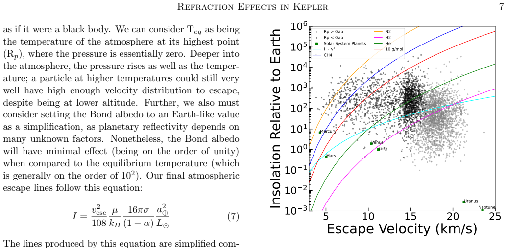
- Atmospheric escape arguments suggest only a subset of above-valley planets can even retain H2, and even that subset shows a heavily damped refraction bump relative to the H/He model.
Reading between the lines
- A sharper version of the paper's own test would inject 2 ppm signals (the claimed amplitude) rather than 10 ppm signals and would exclude the ±0.1 T14 ingress/egress window in the main binned light curves; if the bump survives, the detection is on much firmer ground.
- If the detection is real, the same stacking procedure could be applied in narrow period and radius bins to map where the refraction amplitude turns on, effectively tracing the valley's atmospheric-retention boundary in mean molecular weight.
- The degeneracy between optically thick low-μ and optically thin high-μ atmospheres could be broken by combining the stacked refraction amplitude with transmission-spectroscopy haze measurements for the same population, or by repeating the stack in the infrared where Rayleigh scattering is weaker.
- A testable prediction follows for future large-sample infrared surveys: the above-valley population should show a larger, clearer refraction bump, with an amplitude that depends on wavelength in a way that distinguishes haze damping from genuinely heavy atmospheres.
Editorial analysis
A structured set of objections, weighed in public.
Referee Report
Summary. The paper proposes that a population-level stacking of Kepler DR25 light curves, split by the period-radius valley, can reveal a few-ppm enhancement in out-of-transit flux caused by atmospheric refraction. It detrends and phase-folds KOI light curves, bins them in units of transit duration, compares the binned photometry with RETrO ray-tracing refraction models for fixed mean molecular weights, and then fits mean molecular weight and a vertical offset with MCMC using linear interpolation between the simulated model grid points. The central claim is that the above-valley (APR V) population shows a ~2 ppm out-of-transit bump consistent with mu ≈ 8.8 (+2.3/-0.9) g/mol, while the below-valley (BPR V) population shows no detectable refraction. The authors interpret the result as evidence against common optically thin H/He atmospheres in the APR V population and attribute the damping to clouds and hazes.
Significance. An archival Kepler detection of atmospheric refraction at the 2 ppm level would be a novel population-level probe of exoplanet atmospheres and would complement transmission spectroscopy. The paper has real strengths: it uses the public RETrO simulation suite, performs injection tests to check the pipeline, and includes a random-subsample check showing that the bump is not driven by one subset of the APR V sample. The central result, however, rests on a signal five times smaller than the smallest injected test signal, and the paper does not supply a formal significance for the bump against a flat null. These are fixable with additional analysis, so the result is not yet established but the approach is worth pursuing.
major comments (5)
- [§4 (Injection Tests)] The injection tests only validate recovery of a ~10 ppm peak refraction signal (Figure 3 caption), whereas the APR V detection reported in §5 is ~2 ppm. Because detrending, transit-subtraction, outlier clipping, and binning can in principle have amplitude-dependent effects, recovering a 10 ppm signal does not establish that a 2 ppm signal survives the pipeline. Please rerun the injections with peak amplitudes comparable to 2 ppm, report the recovered amplitude and scatter, and confirm that the shape is preserved.
- [§3.1 / §5] No significance statistic is given for the APR V out-of-transit bump relative to a straight-line (no-refraction) null. The chi-squared values quoted for the discrete 2/4/10/30 g/mol models are not compared to the null for the APR V population, and the MCMC posterior on mu does not by itself tell the reader whether the bump is significantly different from zero. Report a formal delta-chi-squared or bootstrap p-value, with the number of fitted parameters and degrees of freedom, before claiming strong observational evidence.
- [§2 / §4] The main light-curve analysis does not appear to apply the ±0.1 T14 exclusion around ingress/egress that is used in the injection tests to guard against 30-minute-cadence blending. Since the claimed bump peaks close to ingress/egress, transit-model residuals or blending at those phases could mimic the signal. Apply the same exclusion to the main binned APR V and BPR V light curves and show that the 2 ppm bump and the mu = 8.8 g/mol result persist.
- [§3.1] The vertical offset used to compare the binned photometry with the models is manually applied to match the out-of-transit baseline, while the MCMC simultaneously fits a zero-point parameter z. A manual offset is an ad hoc step that can bias the fitted mu and is not part of a statistically self-consistent model. Replace it with a single joint fit of z and mu over the same phase range, or at least demonstrate that the manual offset does not change the posterior by repeating the fit with different baseline choices.
- [§3.1 / Figure 6] For the BPR V population the interpretation is internally inconsistent: the text states that no detection is made, yet the reported chi-squared comparison favors the 30 g/mol model over the null by delta-chi-squared ~10, and the MCMC posterior peaks at mu ~ 212 g/mol, far outside the 2-30 g/mol grid over which the RETrO models were computed. The paper should clarify whether the BPR V data are better described by a heavy atmosphere or by the null model, and state how the interpolation behaves outside the simulated grid.
minor comments (4)
- [Abstract / §5] The abstract and conclusion use strong observational evidence for a ~2 ppm effect whose amplitude is near the binned noise floor; this wording is stronger than the caveats in §3.1 and should be aligned with the reported significance.
- [§3.1] Section 3.1 reports chi-squared values of 91.5, 97.2, 92.3, and 108.1 without degrees of freedom or uncertainties; please provide reduced chi-squared values or the number of data points involved.
- [Figure 6 / §5] The APR V mu posterior is reported as 8.79 (+2.25/-0.94) in Figure 6 but written as 8.8 ± 2.2/0.9 in the text; please use a consistent asymmetric-error notation.
- [Equation (2)] The transit-duration formula in Equation (2) is quoted from Seager & Mallen-Ornelas (2002) via an arXiv e-print entry; please cite the published version of the equation.
Circularity Check
No significant circularity: the claimed refraction detection is a fitted amplitude comparison against external RETrO models, not a prediction derived from its own inputs.
full rationale
The paper's derivation chain is: build binned population light curves from Kepler DR25 PDC photometry; generate RETrO refraction templates using external mean-molecular-weight values; compare templates to the binned data via chi-square and MCMC fits whose free parameters are a vertical zero-point z and the mean molecular weight mu; then interpret the fitted mu. The central number (mu ~8.8 g/mol for APR V) is a fitted parameter, and the conclusion that optically thin H/He atmospheres are not common follows from the discrepancy between the observed ~2 ppm excess and the ~10 ppm 2-4 g/mol templates. That is a model comparison, not an input recycled as an output. The code-level self-citations (Rowe 2015; Rowe 2016; Lissauer et al. 2024) provide methodology, software, or updated parameters rather than importing the result, and RETrO (Dalba 2017) is external. The injection tests are limited to ~10 ppm amplitudes and do not test the Kepler PDC module (Section 4), and the main light curves are not shown with the +/-0.1 T14 ingress/egress exclusion applied in the injection test; these are validation and robustness limitations that belong in a correctness assessment, not circularity. The manual vertical offset in Section 3.1 is another data-processing concern but does not make the fitted mu equal to the conclusion by construction. No equation in the paper defines the detection in terms of the conclusion, and no parameter fitted to the data is renamed as an independent prediction.
Assumptions & free parameters
free parameters (5)
- mean molecular weight (mu) =
APR V: 8.8 (+2.3/-0.9) g/mol; BPR V: 211 (+62/-88) g/mol
- zero point offset (z) =
APR V: 0.24; BPR V: 0.03
- Bond albedo alpha =
0.3
- noise exclusion threshold =
1.5 x expected noise
- RETrO mu simulation grid =
2, 4, 10, 30 g/mol
assumptions (5)
- domain assumption Chen & Kipping (2016) mass-radius relation is used to assign Mp from Rp.
- domain assumption Equilibrium temperature Teq with Bond albedo 0.3 and full stellar heating sets the atmospheric temperature.
- domain assumption Atmospheres are well-mixed, isothermal, optically thin, and haze-free in the RETrO simulations used for interpretation.
- domain assumption The period-radius valley division (Fulton et al.) separates populations with different atmospheric retention.
- domain assumption The ensemble average of thousands of heterogeneous planets reflects a single representative atmosphere, so a single mu can describe the binned light curve.
Cite this review
Pith. "Pith review of Exoplanet Atmospheric Refraction Effects in the Kepler Sample." pith.science (2026). https://pith.science/paper/GFI6URJV
@misc{pith2026250702126,
  author       = {Pith},
  title        = {Pith review of: Exoplanet Atmospheric Refraction Effects in the Kepler Sample},
  year         = {2026},
  howpublished = {\url{https://pith.science/paper/GFI6URJV}},
  note         = {Machine review of arXiv:2507.02126}
}
read the original abstract
We present an analysis on the detection viability of refraction effects in Kepler's exoplanet atmospheres using binning techniques for their light curves in order to compare against simulated refraction effects. We split the Kepler exoplanets into sub-populations according to orbital period and planetary radius, then search for out-of-transit changes in the relative flux associated with atmospheric refraction of starlight. The presence of refraction effects - or lack thereof - may be used to measure and set limits on the bulk properties of an atmosphere, including mean molecular weight or the presence of hazes. In this work, we use the presence of refraction effects to test whether exoplanets above the period-radius valley have H/He atmospheres, which high levels of stellar radiation could evaporate away, in turn leaving rocky cores below the valley. We find strong observational evidence of refraction effects for exoplanets above the period-radius valley based on Kepler photometry, however those related to optically thin H/He atmospheres are not common in the observed planetary population. This result may be attributed to signal dampening caused by clouds and hazes, consistent with the optically thick and intrinsically hotter atmospheres of Kepler exoplanets caused by relatively close host star proximity.
Figures


Figures from the paper (4 more)


Reference graph
Works this paper leans on
-
[1]
, " * write output.state after.block = add.period write newline
ENTRY address archivePrefix author booktitle chapter doi edition editor eprint howpublished institution journal key month note number organization pages publisher school series title misctitle type volume year version url label extra.label sort.label short.list INTEGERS output.state before.all mid.sentence after.sentence after.block FUNCTION init.state.co...
-
[2]
write newline
" write newline "" before.all 'output.state := FUNCTION format.doi doi empty "" "doi:" doi * if FUNCTION format.url url empty "" new.block "" url * "" * if FUNCTION format.eprint eprint empty "" archivePrefix empty "" archivePrefix ":" * if eprint field.or.null * if FUNCTION format.pid eprint empty format.doi format.eprint if FUNCTION n.dashify 't := "" t...
-
[3]
New Grids of ATLAS9 Model Atmospheres
thebibliography [1] 20pt to REFERENCES 6pt =0pt 10pt plus 3pt =0pt =0pt =1pt plus 1pt =0pt =0pt -12pt =13pt plus 1pt =20pt =13pt plus 1pt \@M =10000 =-1.0em =0pt =0pt 0pt =0pt =1.0em @enumiv\@empty 10000 10000 `\.\@m \@noitemerr \@latex@warning Empty `thebibliography' environment \@ifnextchar \@reference \@latexerr Missing key on reference command Each re...
arXiv 2017
-
[4]
Alibert, Y. , Carron, F. , Fortier, A. , et al. 2013, A&A, 558, A109. https://doi.org/10.1051/0004-6361/201321690
-
[5]
Alp, D. , & Demory, B.-O. 2018, A&A, 609, A90. https://doi.org/10.1051/0004-6361/201731484
-
[6]
P., Tollerud , E
Astropy Collaboration , Robitaille , T. P., Tollerud , E. J., et al. 2013, , 558, A33
2013
-
[7]
M., Sip o cz , B
Astropy Collaboration , Price-Whelan , A. M., Sip o cz , B. M., et al. 2018, , 156, 123
2018
-
[8]
M., Lim , P
Astropy Collaboration , Price-Whelan , A. M., Lim , P. L., et al. 2022, , 935, 167
2022
Show all 76 references
-
[9]
2019, The Astrophysical Journal Letters, 887, L14
Benneke, B., Wong, I., Piaulet, C., et al. 2019, The Astrophysical Journal Letters, 887, L14. http://dx.doi.org/10.3847/2041-8213/ab59dc
2019 doi
-
[10]
Borucki , W. J. 2016, Reports on Progress in Physics, 79, 036901
2016
-
[11]
J., Koch , D., Basri , G., et al
Borucki , W. J., Koch , D., Basri , G., et al. 2010, Science, 327, 977
2010
-
[12]
Bétrémieux, Y., & Swain, M. R. 2017, Monthly Notices of the Royal Astronomical Society, 467, 2834. https://doi.org/10.1093/mnras/stx257
2017 doi
-
[13]
C., & Zahnle , K
Catling , D. C., & Zahnle , K. J. 2009, Scientific American, 300, 36
2009
-
[14]
M., Kreidberg, L., et al
Charnay, B., Mendon c a, J. M., Kreidberg, L., et al. 2021, Experimental Astronomy, 53, 417. https://doi.org/10.1007
2021
-
[15]
Chatterjee, S., & Tan, J. C. 2013, 780, 53. https://doi.org/10.1088/0004-637x/780/1/53
2013 doi
-
[16]
2016, The Astrophysical Journal, 834, 17
Chen, J., & Kipping, D. 2016, The Astrophysical Journal, 834, 17. http://dx.doi.org/10.3847/1538-4357/834/1/17
2016 doi
-
[17]
2013, Monthly Notices of the Royal Astronomical Society, 431, 3444
Chiang, E., & Laughlin, G. 2013, Monthly Notices of the Royal Astronomical Society, 431, 3444. https://doi.org/10.1093/mnras/stt424
2013 doi
-
[18]
L., Clarke, B
Christiansen, J. L., Clarke, B. D., Burke, C. J., et al. 2015, 810, 95. https://doi.org/10.1088/0004-637x/810/2/95
2015 doi
-
[19]
Coleman, G. A. L., & Nelson, R. P. 2014, Monthly Notices of the Royal Astronomical Society, 445, 479. https://doi.org/10.1093/mnras/stu1715
2014 doi
-
[20]
Dalba, P. A. 2017, The Astrophysical Journal, 848, 91. http://dx.doi.org/10.3847/1538-4357/aa8e47
2017 doi
-
[21]
2013, Science, 342, 1473–1477
de Wit, J., & Seager, S. 2013, Science, 342, 1473–1477. http://dx.doi.org/10.1126/science.1245450
2013 doi
-
[22]
D., & Charbonneau, D
Dressing, C. D., & Charbonneau, D. 2015, 807, 45. https://doi.org/10.1088/0004-637x/807/1/45
2015 doi
-
[23]
F., Hinsen , K., & Hugunin , J
Dubois , P. F., Hinsen , K., & Hugunin , J. 1996, Computers in Physics, 10, 262
1996
-
[24]
2016, The Journal of Open Source Software, 1, 24
Foreman-Mackey , D. 2016, The Journal of Open Source Software, 1, 24
2016
-
[25]
W., Lang, D., & Goodman, J
Foreman-Mackey, D., Hogg, D. W., Lang, D., & Goodman, J. 2013, Publications of the Astronomical Society of the Pacific, 125, 306–312. http://dx.doi.org/10.1086/670067
2013 doi
-
[26]
2013, 766, 81
Fressin, F., Torres, G., Charbonneau, D., et al. 2013, 766, 81. https://doi.org/10.1088/0004-637x/766/2/81
2013 doi
-
[27]
J., Petigura, E
Fulton, B. J., Petigura, E. A., Howard, A. W., et al. 2017, The Astronomical Journal, 154, 109. http://dx.doi.org/10.3847/1538-3881/aa80eb
2017 doi
-
[28]
Hansen, B. M. S., & Murray, N. 2012, 751, 158. https://doi.org/10.1088/0004-637x/751/2/158
2012 doi
-
[29]
R., Millman , K
Harris , C. R., Millman , K. J., van der Walt , S. J., et al. 2020, , 585, 357
2020
-
[30]
2021, Experimental Astronomy, 53, 323
Helled, R., Werner, S., Dorn, C., et al. 2021, Experimental Astronomy, 53, 323. https://doi.org/10.1007
2021
-
[31]
W., Marcy, G
Howard, A. W., Marcy, G. W., Bryson, S. T., et al. 2012, 201, 15. https://doi.org/10.1088/0067-0049/201/2/15
2012 doi
-
[32]
2002, , 572, 540
Hui , L., & Seager , S. 2002, , 572, 540
2002
-
[33]
Hunter , J. D. 2007, Computing in Science and Engineering, 9, 90
2007
-
[34]
M., He, C., Lewis, N
Hörst, S. M., He, C., Lewis, N. K., et al. 2018, Nature Astronomy, 2, 303–306. http://dx.doi.org/10.1038/s41550-018-0397-0
2018 doi
-
[35]
Ida, S., & Lin, D. N. C. 2004, 604, 388. https://doi.org/10.1086/381724
2004 doi
-
[36]
S., Fegley Jr., B., Schaefer, L., & Ford, E
Kite, E. S., Fegley Jr., B., Schaefer, L., & Ford, E. B. 2020, The Astrophysical Journal, 891, 111. http://dx.doi.org/10.3847/1538-4357/ab6ffb
2020 doi
-
[37]
G., Borucki , W
Koch , D. G., Borucki , W. J., Basri , G., et al. 2010, , 713, L79
2010
-
[38]
2008, Astronomy & Astrophysics, 481, L83–L86
Lecavelier des Etangs, A., Pont, F., Vidal-Madjar, A., & Sing, D. 2008, Astronomy & Astrophysics, 481, L83–L86. http://dx.doi.org/10.1051/0004-6361:200809388
2008 doi
-
[39]
J., & Chiang, E
Lee, E. J., & Chiang, E. 2016, 817, 90. https://doi.org/10.3847/0004-637x/817/2/90
2016 doi
-
[40]
J., Chiang, E., & Ormel, C
Lee, E. J., Chiang, E., & Ormel, C. W. 2014, The Astrophysical Journal, 797, 95. http://dx.doi.org/10.1088/0004-637X/797/2/95
2014 doi
-
[41]
J., Rowe, J
Lissauer, J. J., Rowe, J. F., Jontof-Hutter, D., et al. 2024, The Planetary Science Journal, 5, 152. https://dx.doi.org/10.3847/PSJ/ad0e6e
2024 doi
-
[42]
D., Fortney, J
Lopez, E. D., Fortney, J. J., & Miller, N. 2012, The Astrophysical Journal, 761, 59. http://dx.doi.org/10.1088/0004-637X/761/1/59
2012 doi
-
[43]
D., & Rice, K
Lopez, E. D., & Rice, K. 2018, Monthly Notices of the Royal Astronomical Society, 479, 5303–5311. http://dx.doi.org/10.1093/mnras/sty1707
2018 doi
-
[44]
2002, The Astrophysical Journal, 580, L171–L175
Mandel, K., & Agol, E. 2002, The Astrophysical Journal, 580, L171–L175. http://dx.doi.org/10.1086/345520
2002 doi
-
[45]
2010, in Proceedings of the 9th Python in Science Conference, ed
McKinney , W. 2010, in Proceedings of the 9th Python in Science Conference, ed. S. van der Walt & J. Millman , 56 -- 61
2010
-
[46]
K., & Meadows, V
Misra, A. K., & Meadows, V. S. 2014, The Astrophysical Journal, 795, L14. http://dx.doi.org/10.1088/2041-8205/795/1/L14
2014 doi
-
[47]
, Alibert, Y
Mordasini, C. , Alibert, Y. , & Benz, W. 2009, A&A, 501, 1139. https://doi.org/10.1051/0004-6361/200810301
2009 doi
-
[48]
, Alibert, Y
Mordasini, C. , Alibert, Y. , Georgy, C. , et al. 2012, A&A, 547, A112. https://doi.org/10.1051/0004-6361/201118464
2012 doi
-
[49]
D., & Swift, J
Morton, T. D., & Swift, J. 2014, 791, 10. https://doi.org/10.1088/0004-637x/791/1/10
2014 doi
-
[50]
2022, NASA Exoplanet Archive: A Service of NASA Exoplanet Science Institute , ,
NASA. 2022, NASA Exoplanet Archive: A Service of NASA Exoplanet Science Institute , , . https://exoplanetarchive.ipac.caltech.edu/
2022
-
[51]
Oliphant , T. E. 2007, Computing in Science and Engineering, 9, 10
2007
-
[52]
E., & Wu, Y
Owen, J. E., & Wu, Y. 2013, The Astrophysical Journal, 775, 105. http://dx.doi.org/10.1088/0004-637X/775/2/105
2013 doi
-
[53]
A., Marcy, G
Petigura, E. A., Marcy, G. W., & Howard, A. W. 2013, 770, 69. https://doi.org/10.1088/0004-637x/770/1/69
2013 doi
-
[54]
Piette, A. A. A., & Madhusudhan, N. 2020, The Astrophysical Journal, 904, 154. http://dx.doi.org/10.3847/1538-4357/abbfb1
2020 doi
-
[55]
N., & Cossou, C
Raymond, S. N., & Cossou, C. 2014, Monthly Notices of the Royal Astronomical Society: Letters, 440, L11. https://doi.org/10.1093/mnrasl/slu011
2014 doi
-
[56]
2022, arXiv e-prints, arXiv:2207.05632
Rigby , J., Perrin , M., McElwain , M., et al. 2022, arXiv e-prints, arXiv:2207.05632
2022 arXiv
-
[57]
2016, Kepler: Kepler Transit Model Codebase Release
Rowe , J. 2016, Kepler: Kepler Transit Model Codebase Release. , Zenodo, v1.0, Zenodo, doi:10.5281/zenodo.60297
2016 doi
-
[58]
F., Coughlin, J
Rowe, J. F., Coughlin, J. L., Antoci, V., et al. 2015, The Astrophysical Journal Supplement Series, 217, 16. https://dx.doi.org/10.1088/0067-0049/217/1/16
2015 doi
-
[59]
2002, arXiv e-prints, astro
Seager , S., & Mallen-Ornelas , G. 2002, arXiv e-prints, astro
2002
-
[60]
B., & Deming, D
Sheets, H., Jacob, L., Cowan, N. B., & Deming, D. 2018, A Search for Refraction in Kepler Photometry of Gas Giants, , , arXiv:1809.01189
2018 arXiv
-
[61]
A., & Deming, D
Sheets, H. A., & Deming, D. 2014, The Astrophysical Journal, 794, 133. https://dx.doi.org/10.1088/0004-637X/794/2/133
2014 doi
-
[62]
2017, The Astronomical Journal, 154, 160
---. 2017, The Astronomical Journal, 154, 160. https://dx.doi.org/10.3847/1538-3881/aa88b9
2017 doi
-
[63]
2010, The Astrophysical Journal, 720, 904
Sidis, O., & Sari, R. 2010, The Astrophysical Journal, 720, 904. https://doi.org/10.1088/0004-637x/720/1/904
2010 doi
-
[64]
2020, pandas-dev/pandas: Pandas , vlatest, Zenodo, doi:10.5281/zenodo.3509134
The Pandas Development Team . 2020, pandas-dev/pandas: Pandas , vlatest, Zenodo, doi:10.5281/zenodo.3509134. https://doi.org/10.5281/zenodo.3509134
2020 doi
-
[65]
E., Coughlin, J
Thompson, S. E., Coughlin, J. L., Hoffman, K., et al. 2018, The Astrophysical Journal Supplement Series, 235, 38. http://dx.doi.org/10.3847/1538-4365/aab4f9
2018 doi
-
[66]
E., Coughlin , J
Thompson , S. E., Coughlin , J. L., Hoffman , K., et al. 2018, VizieR Online Data Catalog: Kepler planetary cand. VIII. DR25 reliability (Thompson+, 2018) , VizieR On-line Data Catalog: J/ApJS/235/38. Originally published in: 2018ApJS..235...38T, , , doi:10.26093/cds/vizier.22350038
2018 doi
-
[67]
2021, Ariel: Enabling planetary science across light-years, arXiv, doi:10.48550/ARXIV.2104.04824
Tinetti, G., Eccleston, P., Haswell, C., et al. 2021, Ariel: Enabling planetary science across light-years, arXiv, doi:10.48550/ARXIV.2104.04824. https://arxiv.org/abs/2104.04824
2021 doi
-
[68]
D., Chandrasekaran , H., Jenkins , J
Twicken , J. D., Chandrasekaran , H., Jenkins , J. M., et al. 2010, in Society of Photo-Optical Instrumentation Engineers (SPIE) Conference Series, Vol. 7740, Software and Cyberinfrastructure for Astronomy, ed. N. M. Radziwill & A. Bridger , 77401U
2010
-
[69]
1995 a , Extending and embedding the Python interpreter , Centrum Wiskunde & Informatica
Van Rossum , G. 1995 a , Extending and embedding the Python interpreter , Centrum Wiskunde & Informatica. https://ir.cwi.nl/pub/5006
1995
-
[70]
1995 b , Python tutorial , Centrum Wiskunde & Informatica
---. 1995 b , Python tutorial , Centrum Wiskunde & Informatica. https://ir.cwi.nl/pub/5007
1995
-
[71]
1995 c , Python reference manual , Centrum Wiskunde & Informatica
---. 1995 c , Python reference manual , Centrum Wiskunde & Informatica. https://ir.cwi.nl/pub/5008
1995
-
[72]
1995 d , Python library reference , Centrum Wiskunde & Informatica
---. 1995 d , Python library reference , Centrum Wiskunde & Informatica. https://ir.cwi.nl/pub/5009
1995
-
[73]
E., et al
Virtanen , P., Gommers , R., Oliphant , T. E., et al. 2020, Nature Methods, 17, 261
2020
-
[74]
Youdin, A. N. 2011, 742, 38. https://doi.org/10.1088/0004-637x/742/1/38
2011 doi
-
[75]
2021, Nature Astronomy, 5, 822–831
Yu, X., He, C., Zhang, X., et al. 2021, Nature Astronomy, 5, 822–831. http://dx.doi.org/10.1038/s41550-021-01375-3
2021 doi
-
[76]
J., & Catling, D
Zahnle, K. J., & Catling, D. C. 2017, The Astrophysical Journal, 843, 122. https://doi.org/10.3847\
2017
Reviewed August 6, 2026 · model on record in the stance chip above.
Discussion (0). Continue with ORCID to comment.