REVIEW 2 major objections 3 minor 1 cited by
MALA-within-Gibbs samplers for high-dimensional distributions with sparse conditional structure
T0 review · 2 major / 3 minor · reviewed 2026-08-14 · deepseek-v4-flash
Pith's one-line read MALA-within-Gibbs samplers can keep acceptance, step size, and convergence rate independent of the overall dimension when the target has sparse conditional structure and block-wise log-concavity.
desk verdict A genuinely useful paper on sparse MALA-within-Gibbs, but the main convergence theorem rests on a missing Lipschitz hypothesis and needs a fix before it is citable as proven. read the letter →
The pith
A machine-rendered reading of the paper's core claim, the machinery that carries it, and where it could break.
The reading
What carries the argument
The engine of the argument is sparse conditional structure, Assumption 3.1: the Hessian of the log-target satisfies $\nabla^2_{x_k,x_j}\log\pi(x)=0$ for $k\notin I_j$, with $|I_j|\le S$ and block sizes bounded by $q$, all independent of $m$. This is what makes a block update low-dimensional. On top of it, block-wise log-concavity (Assumption 3.5) gives a uniformly negative matrix $H(x)$ dominating the block Hessian, which provides the contraction constant $\lambda_H$ in the convergence rate. The proof technique is a maximal coupling: two chains share proposal noises $\xi^k_j$, and their accept/reject decisions are coupled through a common uniform variable, which lets the analysis separate the four accept/reject scenarios. The block-distance vector $D^k=(\|x^k_1-z^k_1\|,\ldots,\|x^k_m-z^k_m\|)$ is then shown to satisfy a sparse matrix inequality whose operator norm is bounded by $1-(1-\delta)\lambda_H\tau$ for small $\tau$, giving the dimension-free contraction.
What would settle it
Take a family of block-wise log-concave targets with sparse conditional structure and bounded log-gradients (for instance, densities with support on a fixed bounded cube), keep the block size fixed, and increase the number of blocks $m$ while holding everything else fixed. If the largest step size that keeps the average block acceptance above a chosen threshold decreases with $m$, or if the integrated autocorrelation time per block grows with $m$, then the claimed dimension-independent $\tau_0$ and convergence rate are contradicted. A more targeted check: compute the coupled-contraction factor at a fixed $\tau<\tau_0$ for increasing $m$ and see whether the measured rate approaches $1-(1-\delta)\lambda_H\tau$ uniformly.
Extended reading notes
Core claim
The central discovery is that the dimension dependence of MALA can be moved out of the sampler entirely when the target's log-density has a sparse Hessian. Under Assumption 3.1, each block gradient $v_j(x)=\nabla_{x_j}\log\pi(x)$ depends only on at most $S$ blocks, so a single block update is a genuinely low-dimensional move no matter how large the full vector is. Assumption 3.2 keeps the gradient and its derivatives bounded by dimension-free constants, which makes the acceptance probability at each block close to one in expectation, $E[\alpha_j]\ge 1-M\sqrt{\tau}$, with $M$ independent of $m$. With block-wise log-concavity, Theorem 3.6 gives the convergence rate: for any $\delta>0$ there is $\tau_0>0$ independent of $m$ such that for $\tau<\tau_0$, two coupled MALA-within-Gibbs chains satisfy $$\sum_{i=1}^m \left(E\|x_i^k-z_i^k\|\right)^2 \le \left(1-(1-\delta)\lambda_H\tau\right)^{2k}\sum_{i=1}^m \left(E\|$x_i^{0}$-$z_i^{0}$\|\right)^2.$$ Starting one chain at the target distribution shows the other converges to it at this dimension-free geometric rate. The theorem is an extension, in the paper's reading, of dimension-independent Gibbs convergence for Gaussian targets with sparse precision matrices to a broader class of block-wise log-concave non-Gaussian targets.
Load-bearing premise
The load-bearing premise is Assumption 3.2: the gradient of the log-density and its first derivatives are bounded by constants independent of the overall dimension. The paper itself notes this excludes Gaussian targets, the most natural examples of sparse conditional structure, because their gradients are unbounded; if that boundedness fails, the dimension-independence proof does not apply.
Editorial extensions
If this is right
- For any target satisfying Assumptions 3.1, 3.2, and 3.5, the same step size and per-block acceptance behavior work at dimension $n=mq$ as at small $m$, so tuning does not need to be redone as the number of blocks grows.
- The sampler's mixing time is dimension-free in the sense of the contraction bound: after $k$ Gibbs cycles the worst-case distance to stationarity shrinks by $(1-(1-\delta)\lambda_H\tau)^{2k}$, independent of $m$.
- In Bayesian inverse problems with local prior correlations and local observations, the result says the sampler's speed is governed by the conditional neighborhood size, not by the total state dimension.
- Computational cost per effective sample still scales with the number of blocks if each block update requires a full forward model evaluation; the paper identifies the block-size trade-off between cheaper per-step cost (fewer blocks) and lower autocorrelation (more blocks).
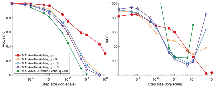
- The numerical experiments show the predicted dimension independence of integrated autocorrelation time and step size in practice, even in a case where block-wise log-concavity is not verified.
Reading between the lines
- Editorial inference: the bounded-gradient assumption is probably not necessary in full strength; since the proof bounds acceptance and contraction locally on the active block set, one could extend the argument to gradients that grow sublinearly in the block size and test numerically whether Gaussian sparse-precision targets, excluded by Assumption 3.2, still show dimension-free acceptance.
- Editorial inference: the result elevates coordinate choice to the main design task; the practical recipe suggested by the paper is to search for coordinates in which the posterior Hessian is approximately sparse (as in the Karhunen-Loève parameterization of the elliptic example), which links the sampler to localization strategies used in data assimilation.
- Editorial inference: the cost formula (integrated autocorrelation time times number of blocks) makes a testable prediction: for a fixed correlation length, the block size minimizing cost per effective sample should be nearly independent of domain size, so the optimum found at $L=16$ should persist at $L=64$ and beyond; this can be checked by experiment.
Signed reviews
Editorial analysis
A structured set of objections, weighed in public.
Referee Report
Summary. The paper studies MALA-within-Gibbs samplers for target distributions with sparse conditional structure. Under Assumption 3.1 (sparse conditional structure), Assumption 3.2 (bounded vector fields), and Assumption 3.5 (block-wise log-concavity), the authors prove Proposition 3.3, a dimension-independent lower bound on block acceptance probabilities, and Theorem 3.6, a dimension-independent geometric contraction rate for two coupled chains. The paper also discusses practical issues of finding a suitable block partition, illustrates the method on a log-Gaussian Cox point process and an elliptic PDE inverse problem, and compares with pCN and MALA/MMALA.
Significance. If the proofs were fully supported, the paper would make a useful contribution: it identifies a natural structural condition under which partial updating can remove the usual dimension dependence of MALA step sizes and convergence rates, complementing earlier Gaussian localization results in [33]. The paper is honestly written, states its assumptions explicitly, and the numerical experiments are substantive and clearly described. The central theorem, however, relies on a lemma that is not justified by the stated hypotheses, so the main contraction result is currently unsupported as written.
major comments (2)
- [Appendix A.4, Lemma A.4] Lemma A.4 is not derivable from Assumption 3.2. Assumption 3.2 contains a Lipschitz bound only for the diagonal Hessian block, ||∇_{x_j} v_j(x) − ∇_{z_j} v_j(z)|| ≤ H_v ||x − z||; for i ≠ j it only asserts the pointwise bound ||∇_{x_i} v_j(x)|| ≤ H_v. Lemma A.4 claims a Lipschitz bound for every mixed block ∇_{x_i} v_j, and its proof applies the diagonal Lipschitz bound to the off-diagonal object ∇_{y_j} v_i(y) − ∇_{z_j} v_i(z). This step is not justified. The gap is load-bearing: Eq. (1.19), used to replace [x^{k,j}, z^{k,j}] by [x^k, z^k], and the estimates on C1 around Eq. (1.25) both rely on Lemma A.4, and these feed directly into the contraction estimate in Theorem 3.6. The authors should either strengthen Assumption 3.2 to include a uniform Lipschitz condition on all mixed Hessian blocks (or a comparable third-derivative condition) and propagate it through the proof, or supply a separate proof of Lemma A.4.
- [Abstract and Section 3.1] The advertised sufficient conditions omit Assumption 3.2. The abstract states that acceptance and step size are dimension-independent when the target has sparse conditional structure and the sampler reflects it; the convergence-rate statement adds only block-wise log-concavity. In fact Proposition 3.3 and Theorem 3.6 also require the bounded-vector-field assumption. This is not a purely cosmetic mismatch: Assumption 3.2 excludes Gaussian targets with sparse precision matrices, the prototypical motivating example discussed in Section 3.1, and it also fails for the log-Gaussian Cox posterior of Section 5.3, whose gradient contains the linear term −[B^{-1}](x − μ1). The authors do acknowledge the restrictiveness of Assumption 3.2, but the abstract and introduction should be revised so that the stated sufficient conditions match the theorem hypotheses, and ideally the paper should discuss what can be proved under weaker growth conditions.
minor comments (3)
- [Appendix A.1, Eq. (1.1)] In the display after Eq. (1.1), the symbol U^n_j appears in the last case; it should presumably be U^k_j.
- [Definition 3.4] The phrase 'uniformly bounded and negative' is slightly misleading because a symmetric negative definite matrix can have positive off-diagonal entries. The definition is clear from the display, but consider saying 'negative definite' and explicitly stating that the off-diagonal entries H_{j,i} may be positive.
- [Section 5.3.3] The discussion of Table 2 states that acceptance ratios are 'independent of the overall problem dimension' based on comparable tuned values. Since step sizes were tuned separately for each block size and problem, it would help to state explicitly that the observed acceptance ratios are comparable after tuning, rather than fixed a priori.
Circularity Check
No significant circularity; proof is self-contained from stated assumptions, with the only caveat being a possible mathematical gap in Lemma A.4, which is not a circularity.
full rationale
The derivation chain is self-contained. Theorem 3.6 is proved from Assumptions 3.1, 3.2, and 3.5 via Lemmas A.1 and A.2, Proposition A.3, and Lemma A.4 in Appendix A; the assumptions are stated at the outset and are not defined in terms of the theorem's conclusion. The dimension-independent acceptance ratio in Proposition 3.3 follows directly from Lemma A.2, and the contraction rate in Theorem 3.6 follows by algebra on block-distance inequalities; no fitted parameters enter the proof. The numerical examples tune step sizes and report IACT, but these are demonstrations of the theory and do not feed back into the assumptions or theorem. The self-citation [33] is used to frame Theorem 3.6 as a generalization of a known Gaussian result and to cite a standard norm bound; none of the argument's load-bearing steps depends on an unverified result from [33]. The only caveat is a possible mathematical gap in Lemma A.4: Assumption 3.2 states a Lipschitz bound only for diagonal Hessian blocks, while Lemma A.4 asserts the same bound for mixed blocks via symmetry; if the missing smoothness is not available, the theorem's proof would need repair. That is a correctness or assumption-strength concern, not circularity, because the claimed conclusion is not an input to the derivation by construction.
Assumptions & free parameters
assumptions (3)
- domain assumption Assumption 3.1: Sparse conditional structure, with known x-independent block index sets I_j of cardinality at most S.
- domain assumption Assumption 3.2: Bounded vector fields, i.e., the gradient of the log density and its derivatives are bounded by constants independent of dimension.
- domain assumption Assumption 3.5: Block-wise log-concavity, a stronger condition than log-concavity, used to prove the dimension-independent convergence rate.
Cite this review
Pith. "Pith review of MALA-within-Gibbs samplers for high-dimensional distributions with sparse conditional structure." pith.science (2026). https://pith.science/paper/GJQ4XLUG
@misc{pith2026190809429,
  author       = {Pith},
  title        = {Pith review of: MALA-within-Gibbs samplers for high-dimensional distributions with sparse conditional structure},
  year         = {2026},
  howpublished = {\url{https://pith.science/paper/GJQ4XLUG}},
  note         = {Machine review of arXiv:1908.09429}
}
read the original abstract
Markov chain Monte Carlo (MCMC) samplers are numerical methods for drawing samples from a given target probability distribution. We discuss one particular MCMC sampler, the MALA-within-Gibbs sampler, from the theoretical and practical perspectives. We first show that the acceptance ratio and step size of this sampler are independent of the overall problem dimension when (i) the target distribution has sparse conditional structure, and (ii) this structure is reflected in the partial updating strategy of MALA-within-Gibbs. If, in addition, the target density is block-wise log-concave, then the sampler's convergence rate is independent of dimension. From a practical perspective, we expect that MALA-within-Gibbs is useful for solving high-dimensional Bayesian inference problems where the posterior exhibits sparse conditional structure at least approximately. In this context, a partitioning of the state that correctly reflects the sparse conditional structure must be found, and we illustrate this process in two numerical examples. We also discuss trade-offs between the block size used for partial updating and computational requirements that may increase with the number of blocks.
Figures

Figures from the paper (4 more)


Forward citations
Cited by 1 Pith paper
-
Analysis of a localised nonlinear Ensemble Kalman Bucy Filter with complete and accurate observations
A localized ensemble Kalman-Bucy filter for nonlinear short-range models has component-wise mean-squared error of order sqrt(ε) independent of state dimension, with pathwise error growing only logarithmically in time.
Reference graph
Works this paper leans on
-
[33]
M. Morzfeld, X. T. Tong, and Y. M. Marzouk. Localization for MCMC: sampling high- dimensional posterior distributions with local structure. J. Comput. Phys. , 310:1–28, 2019
work page 2019
-
[1]
S. Agapiou, O. Papaspiliopoulos, D. Sanz-Alonso, and A.M. Stuart. Importance sampling: computational complexity and intrinsic dimension. Stat. Sci., 32(3):405–431, 2017
work page 2017
-
[2]
M. Asch, M. Bocquet, and M. Nodet. Data assimilation: methods, algorithms and applications . SIAM, 2017
work page 2017
-
[3]
Scalable optimization-based sampling on function space
Johnathan Bardsley, Tiangang Cui, Youssef Marzouk, and Zheng Wang. Scalable optimization- based sampling on function space. arXiv:1903.00870, 2019
work page Pith review arXiv 1903
-
[4]
J. Bear. Modeling groundwater flow and pollution . Kluwer, 1990
work page 1990
- [5]
- [6]
- [7]
Show all 50 references
-
[8]
A stable manifold MCMC method for high dimensions
Alexandros Beskos. A stable manifold MCMC method for high dimensions. Statistics & Probability Letters, 90:46–52, 2014
2014
-
[9]
Bui-Thanh, O
T. Bui-Thanh, O. Ghattas, J. Martin, and G. Stadler. A computational framework for infinite- dimensional Bayesian inverse problems. Part I: The linearized case, with application to global seismic inversion. SIAM J. Sci. Comput. , 36(4):A2494–A2523, 2013
2013
-
[10]
Chen and A
N. Chen and A. J. Majda. Filtering nonlinear turbulent dynamical systems through conditional Gaussian statistics. Mon. Weather Rev., 144(12):4885–4917, 2016
2016
-
[11]
Chen and A
N. Chen and A. J. Majda. Conditional Gaussian systems for multiscale nonlinear stochastic systems: Prediction, state estimation and uncertainty quantification. Entropy, 20(7):509, 2018
2018
-
[12]
N. Chen, A. J. Majda, and X. T. Tong. Spatial localization for nonlinear dynamical stochastic models for excitable media. arXiv:1901.07318
1901 arXiv
-
[13]
N. Chen, A. J. Majda, and X. T. Tong. Rigorous analysis for efficient statistically accurate algorithms for solving Fokker-Plank equations in large dimensions. SIAM-ASA J. Uncertain., 6(3):1198–1223, 2018
2018
-
[14]
Accelerated dimension- independent adaptive Metropolis
Yuxin Chen, David Keyes, Kody JH Law, and Hatem Ltaief. Accelerated dimension- independent adaptive Metropolis. SIAM Journal on Scientific Computing , 38(5):S539–S565, 2016. 23
2016
-
[15]
Chorin and O.H
A.J. Chorin and O.H. Hald. Stochastic tools in mathematics and science . Springer, third edition, 2013
2013
-
[16]
O. F. Christensen, G. O. Roberts, and J. S. Rosenthal. Scaling limits for the transient phase of local Metropolis–Hastings algorithms. J. R. Stat. Soc. B , 67(2):253–268, 2005
2005
-
[17]
S. L. Cotter, G. O. Roberts, A. M. Stuart, and D. White. MCMC methods for functions: modifying old algorithms to make them faster. Stat. Sci., 28(3):424–446, 2013
2013
-
[18]
T. Cui, K. J. H. Law, and Y. M. Marzouk. Dimension-independent likelihood-informed MCMC. J. Comput. Phys. , 304:109–137, 2016
2016
-
[19]
T. Cui, Y. M. Marzouk, and K. Willcox. Scalable posterior approximations for large-scale Bayesian inverse problems via likelihood-informed parameter and state reduction. J. Comput. Phys., 315:363–387, 2016
2016
-
[20]
Dashti and A
M. Dashti and A. Stuart. Uncertainty quantification and weak approximation of an elliptic inverse problem. SIAM J. Numer. Anal. , 49(6):2524–2542, 2011
2011
-
[21]
Edwards, Jonathan Goodman, and Alan D
Robert G. Edwards, Jonathan Goodman, and Alan D. Sokal. Multi-grid Monte Carlo (II). two-dimensional xy model. Nuclear Physics B , 354(2):289 – 327, 1991
1991
-
[22]
Fox and A
C. Fox and A. Parker. Accelerated Gibbs sampling of normal distributions using matrix splittings and polynomials. Bernoulli, 23(4B):3711–3743, 2017
2017
-
[23]
Girolami and B
M. Girolami and B. Calderhead. Riemann manifold Langevin and Hamiltonian Monte Carlo methods. J. R. Stat. Soc. B , 73:123–214, 2011
2011
-
[24]
Random-walk interpretations of classical iteration methods
Jonathan Goodman and Neal Madras. Random-walk interpretations of classical iteration methods. Linear Algebra and its Applications , 216:61–79, 1995
1995
-
[25]
Jonathan Goodman and Alan D. Sokal. Multigrid Monte Carlo method for lattice field theories. Physical Review Letters, 56:1015–1018, 1986
1986
-
[26]
Jonathan Goodman and Alan D. Sokal. Multigrid Monte Carlo method. conceptual founda- tions. Physical Review Letters, 40:2035–2071, Sep 1989
1989
-
[27]
Hairer, A.M
M. Hairer, A.M. Stuart, and S.J. Vollmer. Spectral gaps for a Metropolis–Hastings algorithm in infinite dimensions. Ann. Appl. Probab., 24(6):2455–2490, 2014
2014
-
[28]
A. A. Johnson, G. L. Jones, and R. C. Neath. Component-wise Markov chain Monte Carlo: Uniform and geometric ergodicity under mixing and composition. Stat. Sci. , 28(3):360–375, 08 2013
2013
-
[29]
Adaptive dimension reduction to accelerate infinite-dimensional geometric Markov chain Monte Carlo
Shiwei Lan. Adaptive dimension reduction to accelerate infinite-dimensional geometric Markov chain Monte Carlo. Journal of Computational Physics , 392:71–95, 2019
2019
-
[30]
Graphical models, volume 17
Steffen L Lauritzen. Graphical models, volume 17. Clarendon Press, 1996
1996
-
[31]
Liu and X
Q. Liu and X. T. Tong. Accelerating Metropolis-within-Gibbs sampler with localized compu- tations of differential equations. arXiv:1906.10541, accepted by Statistcs and Computing
1906 arXiv
-
[32]
Møller, A
J. Møller, A. R. Syversveen, and R. P. Waagepetersen. Log Gaussian Cox processes. Scand. J. Stat., 25(3):451–482, 1998. 24
1998
-
[34]
Morzfeld, X
M. Morzfeld, X. Tu, J. Wilkening, and A.J. Chorin. Parameter estimation by implicit sampling. Comm. App. Math. Com. Sci. , 10(2):205–225, 2015
2015
-
[35]
Moselhy and Y.M
T.A. Moselhy and Y.M. Marzouk. Bayesian inference with optimal maps. J. Comput. Phys. , 231:7815–7850, 2012
2012
-
[36]
Neal and G
P. Neal and G. O. Roberts. Optimal scaling for partially updating MCMC algorithms. Ann. Appl. Probab., 16(2):475–515, 05 2006
2006
-
[37]
R. A. Norton and C. Fox. Fast sampling in a linear-Gaussian inverse problem. SIAM-ASA J. Uncertain., 4:1191–1218, 2016
2016
-
[38]
D. S. Oliver, A. C. Reynolds, and N. Liu. Inverse theory for petroleum reservoir characteriza- tion and history matching . Cambridge University Press, 2008
2008
-
[39]
Ottobre, Pillai N.S., Pinski F.J., and A.M
M. Ottobre, Pillai N.S., Pinski F.J., and A.M. Stuart. A function space HMC algorithm with second order Langevin diffusion limit. Bernoulli, 22(1):60–106, 2016
2016
-
[40]
Petra, J
N. Petra, J. Martin, G. Stadler, and O. Ghattas. A computational framework for infinite- dimensional Bayesian inverse problems. Part II: Stochastic Newton MCMC with application to ice sheet flow inverse problems. SIAM J. Sci. Comput. , 36(4):A1525–1555, 2013
2013
-
[41]
Reich and C
S. Reich and C. Cotter. Probabilistic forecasting and Bayesian data assimilation . Cambridge University Press, 2015
2015
-
[42]
G. O. Roberts, A. Gelman, and W. R. Gilks. Weak convergence and optimal scaling of random walk Metropolis algorithms. Ann. Appl. Probab., 7:110–120, 1997
1997
-
[43]
G. O. Roberts and J. S. Rosenthal. Optimal scaling of discrete approximations to Langevin diffusions. J. R. Stat. Soc. B , 60:255–268, 1998
1998
-
[44]
On a generalization of the preconditioned crank–nicolson metropolis algorithm
Daniel Rudolf and Bj¨ orn Sprungk. On a generalization of the preconditioned crank–nicolson metropolis algorithm. Foundations of Computational Mathematics , 18(2):309–343, 2018
2018
-
[45]
A. D. Sokal. Monte Carlo methods in statistical mechanics: foundations and new algorithms, 1998
1998
-
[46]
Spantini, D
A. Spantini, D. Bigoni, and Y. M. Marzouk. Inference via low-dimensional couplings. J. Mach. Learn. Res., 19(66):1–71, 2018
2018
-
[47]
Spantini, A
A. Spantini, A. Solonen, T. Cui, J. Martin, L. Tenorio, and Y. M. Marzouk. Optimal low-rank approximations of Bayesian linear inverse problems. SIAM J. Sci. Comput. , 37(6):A2451– A2487, 2015
2015
-
[48]
S. Vollmer. Dimension-independent MCMC sampling for inverse problems with non-Gaussian priors. SIAM-ASA J. Uncertain. , 3(1):535–561, 2015
2015
-
[49]
U. Wolff. Monte Carlo errors with less errors. Comput. Phys. Commun., 156(2):143–153, 2004
2004
-
[50]
block-update
Olivier Zahm, Tiangang Cui, Kody Law, Alessio Spantini, and Youssef Marzouk. Certified dimension reduction in nonlinear bayesian inverse problems. arXiv:1807.03712, 2018. 25 A Proofs In this appendix, we provide the proofs of Proposition 3.3 and Theorem 3.6. The proof strategy ...
2018 arXiv
Reviewed August 14, 2026 · model on record in the stance chip above.
Discussion (0). Continue with ORCID to comment.