REVIEW 3 major objections 6 minor 2 cited by
Joint Inference of Trajectory and Obstacle in Mean-Field Games via Bilevel Optimization
T0 review · 3 major / 6 minor · reviewed 2026-08-15 · deepseek-v4-flash
Pith's one-line read This paper claims that partial observations of optimal agent trajectories are enough to jointly recover a hidden spatial obstacle and the full optimal paths, with about 0.1 relative L2 error in obstacle reconstruction across low- and…
desk verdict A genuinely new trajectory-based inverse MFG formulation whose headline obstacle-recovery claim is undermined by a regularizer that requires the ground-truth obstacle mass. read the letter →
The pith
A machine-rendered reading of the paper's core claim, the machinery that carries it, and where it could break.
The reading
What carries the argument
The load-bearing object is the bilevel program (15)--(16): an upper-level loss $\frac{1}{KN}\sum_{n=1}^N\sum_{k=1}^K\|F^\ast_k(x_0^n;B)-x_k^n\|_2^2$ matched against trajectory samples, subject to a lower-level minimizer $\theta^\ast$ of the discretized forward mean-field-game loss $\hat L(\theta;\phi)$, which contains kinetic energy, obstacle interaction $\sum_{m,k} B_\phi(F_{\hat\theta_k}(x_m))$, and terminal divergence $D(P_1,F_{\hat\theta_K\#}P_0)$. Trajectories are parametrized as compositions of normalizing-flow maps built from the semigroup property $F_k=f_{\theta_k}\circ\cdots\circ f_{\theta_1}$, and obstacles are parametrized by an MLP $B_\phi$. The penalty method replaces the constraint with $\lambda_P[\hat L(\theta;\phi)-H(\phi)]_+$, and the envelope theorem gives the hypergradient as $\nabla_\phi H(\phi)=\nabla_\phi \hat L(\theta^\ast;\phi)$, so the method never backpropagates through the lower-level optimization dynamics.
What would settle it
Generate trajectories from a forward mean-field game with a ground-truth obstacle $B^\ast$, then run the method with the mass regularizer set to a different value, for example as if $\int_\Omega B^\ast=2$ instead of 1. If the recovered obstacle is not the original up to that scale, or if the relative $L^2$ error jumps far above 0.1, then the scale-normalization assumption is doing essential work. A second check: use trajectories that avoid an entire region and see whether the method correctly reports no obstacle there or instead invents one.
Extended reading notes
Core claim
On the paper's own terms, the central discovery is that the hidden obstacle and the optimal agent trajectories can be inferred jointly from trajectory samples alone, without density measurements or spatial grids. The key is to couple the data-fitting objective to a lower-level variational mean-field-game problem: for a candidate obstacle, the lower level computes the optimal trajectory flow by minimizing kinetic, interaction, and terminal costs, and the upper level then penalizes the mismatch between this flow and the observed trajectories. A mass regularizer pins down the obstacle's scale, and the penalty reformulation with the envelope theorem makes the bilevel program tractable with automatic differentiation. Because the trajectories are represented by normalizing flows rather than a mesh, the method extends to high dimensions where grid-based inverse mean-field-game solvers become intractable.
Load-bearing premise
The method assumes the total amount of obstacle in the domain is known and set to one; if that total is unknown, any obstacle shifted by a constant explains the trajectory data equally well, so the reported recovery accuracy holds only at that chosen scale.
Editorial extensions
If this is right
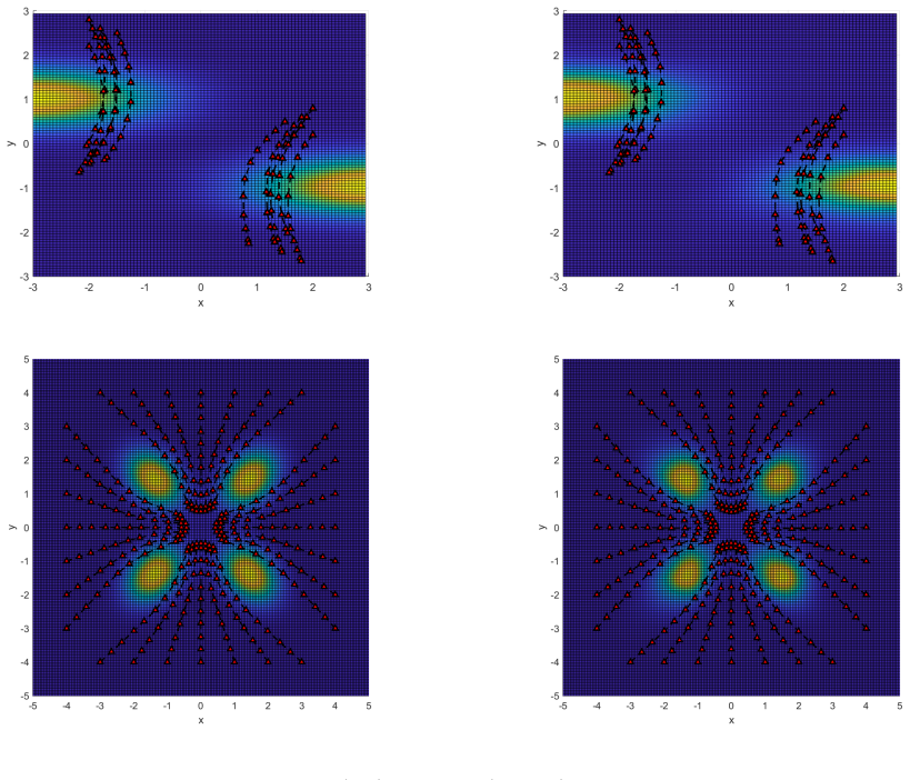
- With trajectory samples only, the obstacle can be recovered at roughly 0.1 relative $L^2$ error across two-bar, flower, cylinder, castle, mountain, and Gaussian obstacle benchmarks.
- Obstacle recovery and trajectory prediction succeed for disjoint and multi-modal obstacles and in dimensions 5 and 10, where mesh-based inverse mean-field-game methods are intractable.
- When training data are scarce (as few as 50 to 3,000 trajectories), the mean-field-regularized bilevel objective generalizes better than plain maximum-likelihood or $L^2$ trajectory fitting, which overfit.
- The bilevel training can be viewed as maximum-likelihood trajectory learning regularized by mean-field-game consistency, so the same method doubles as a regularized trajectory model.
- The mesh-free normalizing-flow parametrization makes the approach applicable to inverse problems in configuration spaces, a setting the paper names as a plausible future application.
Reading between the lines
- The mass regularizer assumes the integral of the true obstacle over the domain is known and normalized to one; absent that knowledge, any constant shift $B^\ast+c$ is indistinguishable from the trajectory data, so the reported relative errors measure recovery of the shape at a preset scale rather than recovery of absolute magnitude.
- Because only the product $\lambda_I B_\phi$ enters the lower-level objective through the interaction cost, the method can be expected to identify obstacle features only in regions that sampled trajectories actually probe, with unsampled regions filled by the MLP's inductive bias rather than by data.
- The same bilevel template could infer other spatially varying mean-field-game parameters, such as drift fields or interaction kernels, by replacing the obstacle network with the appropriate parameterization while keeping the flow-based trajectory representation.
- A natural testable extension is partial-time observation, where each trajectory is seen only on subintervals: the semigroup decomposition should let the upper level match only the observed temporal windows, though obstacle identifiability may degrade accordingly.
Signed reviews
Editorial analysis
A structured set of objections, weighed in public.
Referee Report
Summary. This paper proposes a bilevel-optimization formulation for the joint inverse problem of recovering an unknown obstacle and optimal agent trajectories in a variational mean-field game, given partial observations of optimal trajectories. The lower level is the normalizing-flow-parameterized forward MFG objective (16); the upper level minimizes the squared distance between predicted and observed trajectory points. The authors reformulate the bilevel problem as a penalty problem (20) and add a mass regularizer (21)-(22) to address the additive-constant non-identifiability of the obstacle. They report relative L2 obstacle errors around 0.05-0.15 in 2D, 3D, and up to d=10 experiments, and show improved generalization in a scarce-data regime compared with a trajectory-fitting baseline.
Significance. If the claims are eventually supported, the paper would provide a mesh-free, high-dimensional-capable inverse MFG solver with a practical penalty algorithm. The use of normalizing flows for trajectories, the avoidance of hypergradient backpropagation, and the systematic low-data experiments are useful and go beyond simply applying existing solvers. However, the central obstacle-recovery claim is currently contingent on a regularizer that uses the ground-truth obstacle mass, so the quantitative headline result is not yet established.
major comments (3)
- [Section 3.5, Eqs. (21)-(22)] The mass regularizer R(phi) explicitly uses the ground-truth obstacle integral, R_Omega B*(x) dx, and the paper's own 'Physical Space' paragraph acknowledges that B* is identifiable only up to an additive constant from trajectory data. Since adding a constant c to B* changes the lower-level objective (16) only by a theta-independent constant, observed trajectories cannot distinguish B* from B*+c. The claim that this is 'without loss of generality, because the ground truth obstacle mass can always be normalized to, or regarded as, one' is not valid: rescaling B to have unit mass changes the interaction cost and hence the optimal trajectories, so it is not a free normalization. Consequently the reported relative L2 errors in Tables 1 and 2 and the 'approximately 0.1' claim in the introduction are obtained with an answer-key-dependent prior. In Section 4.1 the Two Bars obstacle has support outside Omega=[-3,3]^2, so the regularizer uses the truncated true mass over Omega, an even more target-specific quantity. The central obstacle-recovery claim is not established unless the authors either estimate the additive constant/mass from data, or reformulate the recoverable quantity as the equivalence class modulo additive constants and report shape errors computed after removing the best constant.
- [Remark 1, Eq. (18)] The claimed equivalence between the maximum-likelihood objective and the upper-level objective in (15) is not generally valid. In a Markovian Gaussian transition model, the negative log-likelihood is, up to constants, sum_{k=0}^{K-1} E[||f_{theta_{k+1}}(x_k) - x_{k+1}||^2], where the conditioning state x_k is the observed intermediate trajectory point. The composition F_{theta_k}(x_0) used in the final expression of Eq. (18) is not equal to the conditional prediction f_{theta_{k+1}}(x_k) unless the model already predicts exactly the observed intermediate states, which is not true during training. Thus the interpretation of (22) as 'regularizing maximum likelihood trajectory learning' is at best an approximation. The derivation should either be corrected by defining the upper objective directly as a trajectory matching loss, or the claim of exact equivalence should be softened.
- [Section 3.4, Eq. (20) and following paragraph] The penalty method relies on the envelope theorem identity grad_phi H(phi) = grad_phi L(theta*; phi) 'for any theta* in argmin'. The lower-level problem (16) is nonconvex because it involves compositions of normalizing flows and an MLP obstacle, and H(phi)=min_theta L(theta;phi) is generally nonsmooth when the argmin is not unique. The identity requires differentiability of the value function and typically uniqueness or at least a regular selection of the optimizer; neither condition is established. If the identity fails, the gradient used in the outer loop is not the true hypergradient. Please state concrete assumptions under which the identity holds, or provide a numerical verification (e.g., comparing the surrogate gradient with a finite-difference hypergradient on a test case).
minor comments (6)
- [Section 3.1] The text reads 'In addition, we assuming the underlying MFG system' and should be 'we assume'; also 'Jeffery's divergence' should be 'Jeffreys divergence'.
- [Equations (11)-(12)] The temporal discretization is stated as 'tk = k Delta t, Delta t = K' which appears to be a typo; it should be Delta t = 1/K to be consistent with the use of Delta t in Eq. (12).
- [Section 4.2, Three Cylinders] In the description of the cylinder obstacle, the notation lists 'mu_2 = (2.5, 2), mu_2 = (-2.5, 2)' where the second 'mu_2' should be 'mu_3'.
- [Figures 5 and 6] The captions for Figures 5 and 6 are identical and end with the incomplete phrase 'as data'; each caption should describe the specific obstacle setting and explain the left and right panels.
- [Section 3.3, flow decomposition] The semi-group notation for the flow maps is confusingly written: after defining Phi^{t_c}_{t_b} composed with Phi^{t_b}_{t_a}, the formula for F_k as a composition of Phi^{t_k}_{t_{k-1}} should be checked and stated more clearly, including the indexing of the flow subnetworks f_{theta_i}.
- [Section 4.4] The baseline is described as 'naive (minimizing l2 trajectory error)', but the upper objective in (15) is also an l2 trajectory error; the distinction between the naive baseline and the proposed method is the penalty term in (20), and this should be stated explicitly.
Circularity Check
Reported obstacle-recovery errors depend on R(phi) injecting the ground-truth obstacle mass; without it, B is identifiable only up to an additive constant.
-
self definitional
[Section 3.5 (Identifiability and Regularization), Eqs. (21)-(22); results in Tables 1-2]
"If we are given any solution (B*,F*) for (11), another solution may be obtained by simply offsetting B* with a constant: (B~*,F*) = (B*+c,F*), which maintains validity on the lower-level. To mitigate this non-uniqueness, we follow typical inverse problem approaches to introduce a regularization. The idea is to match the total mass between the true and parametrized obstacles: R(B) = [ ∫Ω B(x)dx − ∫Ω B*(x)dx / ∫Ω B*(x)dx ]^2 ... We can do this without loss of generality, because the ground truth obstacle mass can always be normalized to, or regarded as, one."
The lower-level objective (16) contains B only through terms of the form λI/(KM) Σ_{m,k} B_phi(F_θk(x_m)); adding a constant c to B_phi adds a θ-independent constant to the loss, so observed trajectories cannot distinguish B from B+c. The regularizer R(B) in Eq. (21) then fixes this non-identifiability by penalizing exactly the difference ∫Ω B_phi dx − ∫Ω B* dx, i.e., by supplying the unknown target obstacle's mass. Calling this 'without loss of generality' is not valid for an inverse problem where ∫Ω B* dx is precisely one of the quantities to be recovered. The headline ~0.1 relative L2 errors in Tables 1 and 2 are therefore computed with an answer-key-dependent prior; they establish shape recovery only up to an additive constant, not the claimed high-fidelity obstacle recovery.
full rationale
The central derivation of the bilevel formulation from the trajectory-based variational MFG is self-contained: the forward problem (6) is a standard variational MFG, and the bilevel reformulation in (10)-(15) follows directly from minimizing trajectory mismatch subject to the lower-level MFG optimality. The learning of trajectories is not circular; the upper-level objective is the negative log-likelihood and the lower-level is the physical MFG cost. However, the obstacle-recovery claim is partially circular because of the mass regularizer R(phi) in Eq. (21)-(22). The paper itself acknowledges that B and B+c produce the same lower-level objective, so trajectories cannot identify the additive constant. The regularizer then injects the true obstacle mass ∫Ω B*(x)dx into the optimization, which is exactly the unknown quantity in a real inverse problem. The phrase 'without loss of generality' is misleading because normalizing the mass presupposes that the true mass is known or recoverable from data, but the data (trajectories) are invariant under constant shifts. Thus, the reported relative L2 errors in Tables 1-2 measure reconstruction with an answer-key-dependent prior; the method does not establish obstacle recovery without that prior. This is a significant circular step, but it is localized to the regularization, not the entire trajectory-inference framework. The self-citations to [33] and [62] are prior work by overlapping authors, but they are used as building blocks (trajectory formulation and bilevel inversion) rather than as a uniqueness theorem that forces the method, so they do not independently raise the circularity score. Overall, the central claim of jointly recovering trajectories and obstacles is partially forced by the mass regularizer, giving a circularity score of 6.
Assumptions & free parameters
free parameters (4)
- obstacle mass prior =
normalized to 1
- MFG cost weights lambda_L, lambda_I, lambda_D =
not reported
- penalty weight lambda_P =
not reported
- mass regularization weight lambda_M =
not reported
assumptions (4)
- domain assumption The MFG admits a variational form (3), i.e., there exist functionals I and M whose variational derivatives give the interaction and terminal costs.
- domain assumption Observed trajectories are exactly optimal for the MFG with the true obstacle.
- domain assumption The flow parametrization with normalizing flows can represent the optimal trajectory maps arbitrarily well.
- ad hoc to paper The envelope theorem applies to the nonconvex lower-level problem (16).
Cite this review
Pith. "Pith review of Joint Inference of Trajectory and Obstacle in Mean-Field Games via Bilevel Optimization." pith.science (2026). https://pith.science/paper/GTTKHFYB
@misc{pith2026250719344,
  author       = {Pith},
  title        = {Pith review of: Joint Inference of Trajectory and Obstacle in Mean-Field Games via Bilevel Optimization},
  year         = {2026},
  howpublished = {\url{https://pith.science/paper/GTTKHFYB}},
  note         = {Machine review of arXiv:2507.19344}
}
read the original abstract
Mean field game (MFG) is an expressive modeling framework for systems with a continuum of interacting agents. While many approaches exist for solving the forward MFG, few have studied its \textit{inverse} problem. In this work, we seek to recover optimal agent trajectories and the unseen spatial obstacle given partial observation on the former. To this end, we use a special type of generative models, normalizing flow, to represent the trajectories and propose a novel formulation of inverse MFG as a bilevel optimization (BLO) problem. We demonstrate the effectiveness of our approach across various MFG scenarios, including those involving multi-modal and disjoint obstacles, highlighting its robustness with respect to obstacle complexity and dimensionality. Alternatively, our formulation can be interpreted as regularizing maximum likelihood trajectory learning with MFG assumptions, which improves generalization performance especially with scarce training data. Impressively, our method also recovers the hidden obstacle with high fidelity in this low-data regime.
Figures


Figures from the paper (3 more)


Forward citations
Cited by 2 Pith papers
-
Truncated Differentiation Through Primal-Dual Solvers for Inverse Potential Mean-Field Games
Truncated backpropagation through the final r PDHG iterations (JFB-r) gives a surrogate-gradient view, converges to the implicit gradient under fixed active-set/exact-detach conditions, and reduces memory/runtime in i...
-
A Globally Convergent Flow for Time-Dependent Mean Field Games and a Solver-Agnostic Framework for Inverse Problems
A discretize-then-flow Hessian-Riemannian method globally converges for time-dependent MFGs while preserving positivity and mass, paired with a solver-agnostic bilevel inverse framework using implicit adjoint differen...
Reference graph
Works this paper leans on
-
[62]
A bilevel optimization method for inverse mean-field games*
Jiajia Yu, Quan Xiao, Tianyi Chen, and Rongjie Lai. A bilevel optimization method for inverse mean-field games*. Inverse Problems, 40(10):105016, sep 2024
work page 2024
-
[1]
Pieter Abbeel, Adam Coates, Morgan Quigley, and Andrew Ng. An application of reinforcement learning to aerobatic helicopter flight.Advances in neural information processing systems, 19, 2006
work page 2006
-
[2]
Apprenticeship learning for motion planning with application to parking lot navigation
Pieter Abbeel, Dmitri Dolgov, Andrew Y Ng, and Sebastian Thrun. Apprenticeship learning for motion planning with application to parking lot navigation. In2008 IEEE/RSJ International Conference on Intelligent Robots and Systems, pages 1083–1090. IEEE, 2008
work page 2008
-
[3]
Apprenticeship learning via inverse reinforcement learning
Pieter Abbeel and Andrew Y Ng. Apprenticeship learning via inverse reinforcement learning. In Proceedings of the twenty-first international conference on Machine learning, page 1, 2004
2004
-
[4]
Inverse reinforcement learning., 2010
Pieter Abbeel and Andrew Y Ng. Inverse reinforcement learning., 2010
work page 2010
-
[5]
Yves Achdou, Francisco J Buera, Jean-Michel Lasry, Pierre-Louis Lions, and Benjamin Moll. Partial differential equation models in macroeconomics.Philosophical Transactions of the Royal Society A: Mathematical, Physical and Engineering Sciences, 372(2028):20130397, 2014
work page 2014
-
[6]
Mean field games: numerical methods.SIAM Journal on Numerical Analysis, 48(3):1136–1162, 2010
Yves Achdou and Italo Capuzzo-Dolcetta. Mean field games: numerical methods.SIAM Journal on Numerical Analysis, 48(3):1136–1162, 2010
2010
-
[7]
Yves Achdou, Jiequn Han, Jean-Michel Lasry, Pierre-Louis Lions, and Benjamin Moll. Income and wealth distribution in macroeconomics: A continuous-time approach.The review of economic studies, 89(1):45–86, 2022
work page 2022
Show all 63 references
-
[8]
A survey of inverse reinforcement learning.Artificial Intelligence Review, 55(6):4307–4346, 2022
Stephen Adams, Tyler Cody, and Peter A Beling. A survey of inverse reinforcement learning.Artificial Intelligence Review, 55(6):4307–4346, 2022
2022
-
[9]
Theory of maxima and the method of lagrange.SIAM Journal on Applied Mathematics, 20(3):343–357, 1971
SN Afriat. Theory of maxima and the method of lagrange.SIAM Journal on Applied Mathematics, 20(3):343–357, 1971
1971
-
[10]
Reinforcement learning for mean field games, with applications to economics.arXiv preprint arXiv:2106.13755, 2021
Andrea Angiuli, Jean-Pierre Fouque, and Mathieu Lauriere. Reinforcement learning for mean field games, with applications to economics.arXiv preprint arXiv:2106.13755, 2021
2021 arXiv
-
[11]
Wasserstein generative adversarial networks
Martin Arjovsky, Soumith Chintala, and Léon Bottou. Wasserstein generative adversarial networks. In International conference on machine learning, pages 214–223. PMLR, 2017
2017
-
[12]
A survey of inverse reinforcement learning: Challenges, methods and progress
Saurabh Arora and Prashant Doshi. A survey of inverse reinforcement learning: Challenges, methods and progress. Artificial Intelligence, 297:103500, 2021
2021
-
[13]
A computational fluid mechanics solution to the monge- kantorovich mass transfer problem.Numerische Mathematik, 84(3):375–393, 2000
Jean-David Benamou and Yann Brenier. A computational fluid mechanics solution to the monge- kantorovich mass transfer problem.Numerische Mathematik, 84(3):375–393, 2000. 14
2000
-
[14]
Augmented lagrangian methods for transport optimization, mean-field games and degenerate pdes.Journal of Optimization Theory and Applications, 167:1–26, 2015
Jean-David Benamou and Guillaume Carlier. Augmented lagrangian methods for transport optimization, mean-field games and degenerate pdes.Journal of Optimization Theory and Applications, 167:1–26, 2015
2015
-
[15]
Variational mean field games
Jean-David Benamou, Guillaume Carlier, and Filippo Santambrogio. Variational mean field games. In Active Particles, Volume 1, pages 141–171. Springer, 2017
2017
-
[16]
Monte carlo and quasi-monte carlo methods.Acta numerica, 7:1–49, 1998
Russel E Caflisch. Monte carlo and quasi-monte carlo methods.Acta numerica, 7:1–49, 1998
1998
-
[17]
Mean field game of controls and an application to trade crowding
Pierre Cardaliaguet and Charles-Albert Lehalle. Mean field game of controls and an application to trade crowding. Mathematics and Financial Economics, 12(3):335–363, 2018
2018
-
[18]
Individual-level inverse reinforcement learning for mean field games.arXiv preprint arXiv:2202.06401, 2022
Yang Chen, Libo Zhang, Jiamou Liu, and Shuyue Hu. Individual-level inverse reinforcement learning for mean field games.arXiv preprint arXiv:2202.06401, 2022
2022 arXiv
-
[19]
A numerical algorithm for inverse problem from partial boundary measurement arising from mean field game problem.Inverse Problems, 39(1):014001, 2022
Yat Tin Chow, Samy Wu Fung, Siting Liu, Levon Nurbekyan, and Stanley Osher. A numerical algorithm for inverse problem from partial boundary measurement arising from mean field game problem.Inverse Problems, 39(1):014001, 2022
2022
-
[20]
Fast and accurate deep network learning by exponential linear units (elus).arXiv preprint arXiv:1511.07289, 2015
Djork-Arné Clevert, Thomas Unterthiner, and Sepp Hochreiter. Fast and accurate deep network learning by exponential linear units (elus).arXiv preprint arXiv:1511.07289, 2015
2015 arXiv
-
[21]
Sinkhorn distances: Lightspeed computation of optimal transport.Advances in neural information processing systems, 26:2292–2300, 2013
Marco Cuturi. Sinkhorn distances: Lightspeed computation of optimal transport.Advances in neural information processing systems, 26:2292–2300, 2013
2013
-
[22]
A mean field game inverse problem.Journal of Scientific Computing, 92(1):7, 2022
Lisang Ding, Wuchen Li, Stanley Osher, and Wotao Yin. A mean field game inverse problem.Journal of Scientific Computing, 92(1):7, 2022
2022
-
[23]
Nice: Non-linear independent components estimation
Laurent Dinh, David Krueger, and Yoshua Bengio. Nice: Non-linear independent components estimation. arXiv preprint arXiv:1410.8516, 2014
2014 arXiv
-
[24]
Density estimation using real nvp.arXiv preprint arXiv:1605.08803, 2016
Laurent Dinh, Jascha Sohl-Dickstein, and Samy Bengio. Density estimation using real nvp.arXiv preprint arXiv:1605.08803, 2016
2016 arXiv
-
[25]
Neural spline flows.Advances in Neural Information Processing Systems, 32:7511–7522, 2019
Conor Durkan, Artur Bekasov, Iain Murray, and George Papamakarios. Neural spline flows.Advances in Neural Information Processing Systems, 32:7511–7522, 2019
2019
-
[26]
An optimal execution problem in finance targeting the market trading speed: An mfg formulation
Dena Firoozi and Peter E Caines. An optimal execution problem in finance targeting the market trading speed: An mfg formulation. In2017 IEEE 56th Annual Conference on Decision and Control (CDC), pages 7–14. IEEE, 2017
2017
-
[27]
Generative adversarial nets.Advances in neural information processing systems, 27, 2014
Ian Goodfellow, Jean Pouget-Abadie, Mehdi Mirza, Bing Xu, David Warde-Farley, Sherjil Ozair, Aaron Courville, and Yoshua Bengio. Generative adversarial nets.Advances in neural information processing systems, 27, 2014
2014
-
[28]
Mean field games and applications
Olivier Guéant, Jean-Michel Lasry, and Pierre-Louis Lions. Mean field games and applications. In Paris-Princeton lectures on mathematical finance 2010, pages 205–266. Springer, 2011
2010
-
[29]
Decoding mean field games from population and environment observations by gaussian processes.Journal of Computational Physics, 508:112978, 2024
Jinyan Guo, Chenchen Mou, Xianjin Yang, and Chao Zhou. Decoding mean field games from population and environment observations by gaussian processes.Journal of Computational Physics, 508:112978, 2024
2024
-
[30]
Learning mean-field games.Advances in Neural Information Processing Systems, 32, 2019
Xin Guo, Anran Hu, Renyuan Xu, and Junzi Zhang. Learning mean-field games.Advances in Neural Information Processing Systems, 32, 2019
2019
-
[31]
Flow++: Improving flow-based generative models with variational dequantization and architecture design
Jonathan Ho, Xi Chen, Aravind Srinivas, Yan Duan, and Pieter Abbeel. Flow++: Improving flow-based generative models with variational dequantization and architecture design. InInternational Conference on Machine Learning, pages 2722–2730. PMLR, 2019
2019
-
[32]
Neural autoregressive flows
Chin-Wei Huang, David Krueger, Alexandre Lacoste, and Aaron Courville. Neural autoregressive flows. In International Conference on Machine Learning, pages 2078–2087. PMLR, 2018. 15
2018
-
[33]
Bridging mean-field games and normalizing flows with trajectory regularization.Journal of Computational Physics, 487:112155, 2023
Han Huang, Jiajia Yu, Jie Chen, and Rongjie Lai. Bridging mean-field games and normalizing flows with trajectory regularization.Journal of Computational Physics, 487:112155, 2023
2023
-
[34]
Large-population cost-coupled lqg problems with nonuniform agents: individual-mass behavior and decentralizedε-nash equilibria
Minyi Huang, Peter E Caines, and Roland P Malhamé. Large-population cost-coupled lqg problems with nonuniform agents: individual-mass behavior and decentralizedε-nash equilibria. IEEE transactions on automatic control, 52(9):1560–1571, 2007
2007
-
[35]
Minyi Huang, Roland P Malhamé, Peter E Caines, et al. Large population stochastic dynamic games: closed-loop mckean-vlasov systems and the nash certainty equivalence principle.Communications in Information & Systems, 6(3):221–252, 2006
2006
-
[36]
Solving large-scale optimization problems with a convergence rate independent of grid size.SIAM Journal on Numerical Analysis, 57(3):1100–1123, 2019
Matt Jacobs, Flavien Léger, Wuchen Li, and Stanley Osher. Solving large-scale optimization problems with a convergence rate independent of grid size.SIAM Journal on Numerical Analysis, 57(3):1100–1123, 2019
2019
-
[37]
Hands-on bayesian neural networks—a tutorial for deep learning users.IEEE Computational Intelligence Magazine, 17(2):29–48, 2022
Laurent Valentin Jospin, Hamid Laga, Farid Boussaid, Wray Buntine, and Mohammed Bennamoun. Hands-on bayesian neural networks—a tutorial for deep learning users.IEEE Computational Intelligence Magazine, 17(2):29–48, 2022
2022
-
[38]
Adam: A method for stochastic optimization.arXiv preprint arXiv:1412.6980, 2014
Diederik P Kingma and Jimmy Ba. Adam: A method for stochastic optimization.arXiv preprint arXiv:1412.6980, 2014
2014 arXiv
-
[39]
Auto-encoding variational bayes.arXiv preprint arXiv:1312.6114, 2013
Diederik P Kingma and Max Welling. Auto-encoding variational bayes.arXiv preprint arXiv:1312.6114, 2013
2013 arXiv
-
[40]
Improved variational inference with inverse autoregressive flow.Advances in neural information processing systems, 29:4743–4751, 2016
Durk P Kingma, Tim Salimans, Rafal Jozefowicz, Xi Chen, Ilya Sutskever, and Max Welling. Improved variational inference with inverse autoregressive flow.Advances in neural information processing systems, 29:4743–4751, 2016
2016
-
[41]
Normalizing flows: An introduction and review of current methods
Ivan Kobyzev, Simon Prince, and Marcus Brubaker. Normalizing flows: An introduction and review of current methods. IEEE Transactions on Pattern Analysis and Machine Intelligence, 2020
2020
-
[42]
Efficiency of the price formation process in presence of high frequency participants: a mean field game analysis
Aimé Lachapelle, Jean-Michel Lasry, Charles-Albert Lehalle, and Pierre-Louis Lions. Efficiency of the price formation process in presence of high frequency participants: a mean field game analysis. Mathematics and Financial Economics, 10(3):223–262, 2016
2016
-
[43]
Mean field games.Japanese journal of mathematics, 2(1):229– 260, 2007
Jean-Michel Lasry and Pierre-Louis Lions. Mean field games.Japanese journal of mathematics, 2(1):229– 260, 2007
2007
-
[44]
Scalable deep reinforcement learning algorithms for mean field games
Mathieu Laurière, Sarah Perrin, Sertan Girgin, Paul Muller, Ayush Jain, Theophile Cabannes, Georgios Piliouras, Julien Pérolat, Romuald Élie, Olivier Pietquin, et al. Scalable deep reinforcement learning algorithms for mean field games. InInternational Conference on Machine Le...
2022
-
[45]
Alex Tong Lin, Samy Wu Fung, Wuchen Li, Levon Nurbekyan, and Stanley J. Osher. Alternating the population and control neural networks to solve high-dimensional stochastic mean-field games. Proceedings of the National Academy of Sciences, 118(31):e2024713118, 2021
2021
-
[46]
Risheng Liu, Jiaxin Gao, Jin Zhang, Deyu Meng, and Zhouchen Lin. Investigating bi-level optimization for learning and vision from a unified perspective: A survey and beyond.IEEE Transactions on Pattern Analysis and Machine Intelligence, 44(12):10045–10067, 2021
2021
-
[47]
Towards gradient-based bilevel optimization with non-convex followers and beyond.Advances in Neural Information Processing Systems, 34:8662–8675, 2021
Risheng Liu, Yaohua Liu, Shangzhi Zeng, and Jin Zhang. Towards gradient-based bilevel optimization with non-convex followers and beyond.Advances in Neural Information Processing Systems, 34:8662–8675, 2021
2021
-
[48]
A general descent aggregation framework for gradient-based bi-level optimization.IEEE Transactions on Pattern Analysis and Machine Intelligence, 45(1):38–57, 2022
Risheng Liu, Pan Mu, Xiaoming Yuan, Shangzhi Zeng, and Jin Zhang. A general descent aggregation framework for gradient-based bi-level optimization.IEEE Transactions on Pattern Analysis and Machine Intelligence, 45(1):38–57, 2022. 16
2022
-
[49]
A mean field game approach to swarming robots control
Zhiyu Liu, Bo Wu, and Hai Lin. A mean field game approach to swarming robots control. In2018 Annual American Control Conference (ACC), pages 4293–4298. IEEE, 2018
2018
-
[50]
Mish: A self regularized non-monotonic activation function
Diganta Misra. Mish: A self regularized non-monotonic activation function. arXiv preprint arXiv:1908.08681, 2019
1908 arXiv
-
[51]
Optimal transport with proximal splitting
Nicolas Papadakis, Gabriel Peyré, and Edouard Oudet. Optimal transport with proximal splitting. SIAM Journal on Imaging Sciences, 7(1):212–238, 2014
2014
-
[52]
Masked autoregressive flow for density estimation
George Papamakarios, Theo Pavlakou, and Iain Murray. Masked autoregressive flow for density estimation. arXiv preprint arXiv:1705.07057, 2017
2017 arXiv
-
[53]
On identifiability of parametric statistical models
Carlos Daniel Mimoso Paulino and Carlos Alberto de Bragança Pereira. On identifiability of parametric statistical models. Journal of the Italian Statistical Society, 3:125–151, 1994
1994
-
[54]
Computational optimal transport: With applications to data science
Gabriel Peyré and Marco Cuturi. Computational optimal transport: With applications to data science. Foundations and Trends in Machine Learning, 11(5-6):355–607, 2019
2019
-
[55]
Tarek Rakha and Alice Gorodetsky. Review of unmanned aerial system (uas) applications in the built environment: Towards automated building inspection procedures using drones.Automation in Construction, 93:252–264, 2018
2018
-
[56]
Learning agents for uncertain environments
Stuart Russell. Learning agents for uncertain environments. InProceedings of the eleventh annual conference on Computational learning theory, pages 101–103, 1998
1998
-
[57]
A machine learning framework for solving high-dimensional mean field game and mean field control problems.Proceedings of the National Academy of Sciences, 117(17):9183–9193, 2020
Lars Ruthotto, Stanley J Osher, Wuchen Li, Levon Nurbekyan, and Samy Wu Fung. A machine learning framework for solving high-dimensional mean field game and mean field control problems.Proceedings of the National Academy of Sciences, 117(17):9183–9193, 2020
2020
-
[58]
Mean-field games for bio-inspired collective decision-making in dynamical networks.arXiv preprint arXiv:1802.03435, 2018
Leonardo Stella and Dario Bauso. Mean-field games for bio-inspired collective decision-making in dynamical networks.arXiv preprint arXiv:1802.03435, 2018
2018 arXiv
-
[59]
Unconstrained monotonic neural networks.Advances in Neural Information Processing Systems, 32:1545–1555, 2019
Antoine Wehenkel and Gilles Louppe. Unconstrained monotonic neural networks.Advances in Neural Information Processing Systems, 32:1545–1555, 2019
2019
-
[60]
Computational mean-field games on manifolds
Jiajia Yu, Rongjie Lai, Wuchen Li, and Stanley Osher. Computational mean-field games on manifolds. Journal of Computational Physics, 484:112070, 2023
2023
-
[61]
A fast proximal gradient method and convergence analysis for dynamic mean field planning.Mathematics of Computation, 93(346):603–642, 2024
Jiajia Yu, Rongjie Lai, Wuchen Li, and Stanley Osher. A fast proximal gradient method and convergence analysis for dynamic mean field planning.Mathematics of Computation, 93(346):603–642, 2024
2024
-
[63]
Learning surrogate potential mean field games via gaussian processes: A data-driven approach to ill-posed inverse problems, 2025
Jingguo Zhang, Xianjin Yang, Chenchen Mou, and Chao Zhou. Learning surrogate potential mean field games via gaussian processes: A data-driven approach to ill-posed inverse problems, 2025. 17
2025
Reviewed August 15, 2026 · model on record in the stance chip above.
Discussion (0). Continue with ORCID to comment.